Welcome
Hello, I'm Mahmoud, and these are my notes. Since you're reading something I've written, I want to share a bit about how I approach learning and what you can expect here.
Want to know more about me? Check out my blog at mahmoud.ninja
My Philosophy
I believe there are no shortcuts to success. To me, success means respecting your time, and before investing that time, you need a plan rooted in where you want to go in life.
Learn, learn, learn, and when you think you've learned enough, write it down and share it.
About These Notes
I don't strive for perfectionism. Sometimes I write something and hope someone will point out where I'm wrong so we can both learn from it. That's the beauty of sharing knowledge: it's a two-way street.
I tend to be pretty chill, and I occasionally throw in some sarcasm when it feels appropriate. These are my notes after all, so please don't be annoyed if you encounter something that doesn't resonate with you, just skip ahead.
I'm creating this resource purely out of love for sharing and teaching. Ironically, I'm learning more by organizing and explaining these concepts than I ever did just studying them. Sharing is learning. Imagine if scientists never shared their research, we'd still be in the dark ages.
Licensing & Copyright
Everything I create here is released under Creative Commons (CC BY 4.0). You're free to share, copy, remix, and build upon this material for any purpose, even commercially, as long as you give appropriate credit.
Important Legal Notice
I deeply respect intellectual property rights. I will never share copyrighted materials, proprietary resources, or content that was shared with our class under restricted access. All external resources linked here are publicly available or properly attributed.
If you notice any copyright violations or improperly shared materials, please contact me immediately at mahmoudahmedxyz@gmail.com, and I will remove the content right away and make necessary corrections.
Final Thoughts
I have tremendous respect for everyone in this learning journey. We're all here trying to understand complex topics, and we all learn differently. If these notes help you even a little bit, then this project has served its purpose.
Linux Fundamentals
The History of Linux
In 1880, the French government awarded the Volta Prize to Alexander Graham Bell. Instead of going to the Maldives (kidding...he had work to do), he went to America and opened Bell Labs.
This lab researched electronics and something revolutionary called the mathematical theory of communications. In the 1950s came the transistor revolution. Bell Labs scientists won 10 Nobel Prizes...not too shabby.
But around this time, Russia made the USA nervous by launching the first satellite, Sputnik, in 1957. This had nothing to do with operating systems, it was literally just a satellite beeping in space, but it scared America enough to kickstart the space race.
President Eisenhower responded by creating ARPA (Advanced Research Projects Agency) in 1958, and asked James Killian, MIT's president, to help develop computer technology. This led to Project MAC (Mathematics and Computation) at MIT.
Before Project MAC, using a computer meant bringing a stack of punch cards with your instructions, feeding them into the machine, and waiting. During this time, no one else could use the computer, it was one job at a time.
The big goal of Project MAC was to allow multiple programmers to use the same computer simultaneously, executing different instructions at the same time. This concept was called time-sharing.
MIT and Bell Labs cooperated and developed the first operating system to support time-sharing: CTSS (Compatible Time-Sharing System). They wanted to expand this to larger mainframe computers, so they partnered with General Electric (GE), who manufactured these machines. In 1964, they developed the first real OS with time-sharing support called Multics. It also introduced the terminal as a new type of input device.
In the late 1960s, GE and Bell Labs left the project. GE's computer department was bought by Honeywell, which continued the project with MIT and created a commercial version that sold for 25 years.
In 1969, Bell Labs engineers (Dennis Ritchie and Ken Thompson) developed a new OS based on Multics. In 1970, they introduced Unics (later called Unix, the name was a sarcastic play on "Multics," implying it was simpler).
The first two versions of Unix were written in assembly language, which was then translated by an assembler and linker into machine code. The big problem with assembly was that it was tightly coupled to specific processors, meaning you'd need to rewrite Unix for each processor architecture. So Dennis Ritchie decided to create a new programming language: C.
They rebuilt Unix using C. At this time, AT&T owned Bell Labs (now it's Nokia). AT&T declared that Unix was theirs and no one else could touch it, classic monopolization.
AT&T did make one merciful agreement: universities could use Unix for educational purposes. But after AT&T was broken up into smaller companies in 1984, even this stopped. Things got worse.
One person was watching all this and decided to take action: Andrew S. Tanenbaum. In 1987, he created a new Unix-inspired OS called MINIX. It was free for universities and designed to work on Intel chips. It had some issues, occasional crashes and overheating, but this was just the beginning. This was the first time someone made a Unix-like OS outside of AT&T.
The main difference between Unix and MINIX was that MINIX was built on a microkernel architecture. Unix had a larger monolithic kernel, but MINIX separated some modules, for example, device drivers were moved from kernel space to user space.
It's unclear if MINIX was truly open source, but people outside universities wanted access and wanted to contribute and modify it.
Around the same time MINIX was being developed, another person named Richard Stallman started the free software movement based on four freedoms: Freedom to run, Freedom to study, Freedom to modify, and Freedom to share. This led to the GPL license (GNU General Public License), which ensured that if you used something free, your product must also be free. They created the GNU Project, which produced many important tools like the GCC compiler, Bash shell, and more.
But there was one problem: the kernel, the beating heart of the operating system that talks to the hardware, was missing.
Let's leave the USA and cross the Atlantic Ocean. In Finland, a student named Linus Torvalds was stuck at home while his classmates vacationed in Baltim Egypt (kidding). He was frustrated with MINIX, had heard about GPL and GNU, and decided to make something new. "I know what I should do with my life," he thought. As a side hobby project in 1991, he started working on a new kernel (not based on MINIX) and sent an email to his classmates discussing it.
Linus announced Freax (maybe meant "free Unix") with a GPL license. After six months, he released another version and called it Linux. He improved the kernel and integrated many GNU Project tools. He uploaded the source code to the internet (though Git came much later, he initially used FTP). This mini-project became the most widely used OS on Earth.
The penguin mascot (Tux) came from multiple stories: Linus was supposedly bitten by a penguin at a zoo, and he also watched March of the Penguins and was inspired by how they cooperate and share to protect their eggs and each other. Cute and fitting.
...And that's the history intro.
Linux Distributions
Okay... let's install Linux. Which Linux? Wait, really? There are multiple Linuxes?
Here's the deal: the open-source part is the kernel, but different developers take it and add their own packages, libraries, and maybe create a GUI. Others add their own tweaks and features. This leads to many different versions, which we call distributions (or distros for short).
Some examples: Red Hat, Slackware, Debian.
Even distros themselves can be modified with additional features, which creates a version of a version. For example, Debian led to Ubuntu, these are called derivatives.
How many distros and derivatives exist in the world? Many. How many exactly? I said many. Anyone with a computer can create one.
So what's the main difference between these distros, so I know which one is suitable for me? The main differences fall into two categories: philosophical and technical.
One of the biggest technical differences is package management, the system that lets you install software, including the type and format of software itself.
Another difference is configuration files, their locations differ from one distro to another.
We agreed that everything is free, right? Well, you may find some paid versions like Red Hat Enterprise Linux, which charges for features like an additional layer of security, professional support, and guaranteed upgrades. Fedora is also owned by Red Hat and acts as a testing ground (a "backdoor," if you will) for new features before they hit Red Hat Enterprise.
The philosophical part is linked to the functional part. If you're using Linux for research, there are distros with specialized software for that. Maybe you're into ethical hacking, Kali Linux is for you. If you're afraid of switching from another OS, you might like Linux Mint, which even has themes that make it look like Windows.
Okay, which one should I install now? Heh... There are a ton of options and you can install any of them, but my preference is Ubuntu.
Ubuntu is the most popular for development and data engineering. But remember, in all cases, you'll be using the terminal a lot. So install Ubuntu, maybe in dual boot, and keep Windows if possible so you don't regret it later and blame me.
The Terminal
Yes, this is what matters for us. Every distro will come with a default terminal but you can install others if you want. Anyway, open the terminal from the apps or just click Ctrl+Alt+T.

Zoom in using Ctrl+Shift++ or out using Ctrl+-
By default first thing you will see the prompt name@host:path$ which your name @ the machine name then ~ then dollar sign colon then $. After $ you can write your command.
You can change the colors and all preferences and save each for profile.
You can even change the prompt itself as it is just a variable (more on variable later).
Basic Commands
First, everything is case sensitive, so be careful.
[1] echo
This command echoes whatever you write after it.
$ echo "Hello, terminal"
Output:
Hello, terminal
[2] pwd
This prints the current directory.
$ pwd
Output:
/home/mahmoudxyz
[3] cd
This is for changing the directory.
$ cd Desktop
The directory changed with no output, you can check this using pwd.
To go back to the main directory use:
$ cd ~
Or just:
$ cd
Note that this means we are back to /home/mahmoudxyz
To go back to the previous directory (in this case /home) even if you don't know the name, you can use:
$ cd ..
[4] ls
This command outputs the current files and directories (folders).
First let's go to desktop again:
$ cd /home/mahmoudxyz/Desktop
Yes, you can go to a specific dir if you know its path. Note that in Linux we are using / not \ like Windows.
Now let's see what files and directories are in my Desktop:
$ ls
Output:
file1 python testdir
If you notice that in my case, my terminal supports colors. The blue ones are directories and the grey (maybe black) is the file.
But you may deal with some terminal that doesn't support colors, in this case you can use:
$ ls -F
Output:
file1 python/ testdir/
What ends with / like python/ is a directory otherwise it's a file like file1.
You can see the hidden files using:
$ ls -a
Output:
. .. file1 python testdir .you-cant-see-me
We saw .you-cant-see-me, but we are not hackers that we saw something hidden, being hidden is more than organizing purpose than actually hiding something.
You can also list the files in the long format using:
$ ls -l
Output:
total 8
-rw-rw-r-- 1 mahmoudxyz mahmoudxyz    0 Nov  2 10:48 file1
drwxrwxr-x 2 mahmoudxyz mahmoudxyz 4096 Oct 16 15:20 python
drwxrwxr-x 2 mahmoudxyz mahmoudxyz 4096 Nov  1 21:45 testdir
Let's take the file1 and analyze the output:
| Column | Meaning |
|---|---|
-rw-rw-r-- 1 | File type + permissions (more on this later) |
1 | Number of hard links (more on this later) |
mahmoudxyz | Owner name |
mahmoudxyz | Group name |
0 | File size (bytes) |
Nov 2 10:48 | Last modification date & time |
file1 | File or directory name |
We can also combine these flags/options:
$ ls -l -a -F
Output:
total 16
drwxr-xr-x  4 mahmoudxyz mahmoudxyz 4096 Nov  2 10:53 ./
drwxr-x--- 47 mahmoudxyz mahmoudxyz 4096 Nov  1 21:55 ../
-rw-rw-r--  1 mahmoudxyz mahmoudxyz    0 Nov  2 10:48 file1
drwxrwxr-x  2 mahmoudxyz mahmoudxyz 4096 Oct 16 15:20 python/
drwxrwxr-x  2 mahmoudxyz mahmoudxyz 4096 Nov  1 21:45 testdir/
-rw-rw-r--  1 mahmoudxyz mahmoudxyz    0 Nov  2 10:53 .you-cant-see-me
Or shortly:
$ ls -laF
The same output. The order of options is not important so ls -lFa will work as well.
[5] clear
This cleans your terminal. You can also use shortcut Ctrl+l
[6] mkdir
This makes a new directory.
$ mkdir new-dir
Then let's see the output:
$ ls -F
Output:
file1 new-dir/ python/ testdir/
[7] rmdir
This will remove the directory.
$ rmdir new-dir
Then let's see the output:
$ ls -F
Output:
file1 python/ testdir/
[8] touch
This command is for creating a new file.
$ mkdir new-dir
$ cd new-dir
$ touch file1
$ ls -l
Output:
total 0
-rw-rw-r-- 1 mahmoudxyz mahmoudxyz 0 Nov  2 11:26 file1
You can also make more than one file with:
$ touch file2 file3
$ ls -l
Output:
total 0
-rw-rw-r-- 1 mahmoudxyz mahmoudxyz 0 Nov  2 11:26 file1
-rw-rw-r-- 1 mahmoudxyz mahmoudxyz 0 Nov  2 11:28 file2
-rw-rw-r-- 1 mahmoudxyz mahmoudxyz 0 Nov  2 11:28 file3
In fact touch was created for modifying the timestamp of the file so let's try again:
$ touch file1
$ ls -l
Output:
total 0
-rw-rw-r-- 1 mahmoudxyz mahmoudxyz 0 Nov  2 11:30 file1
-rw-rw-r-- 1 mahmoudxyz mahmoudxyz 0 Nov  2 11:28 file2
-rw-rw-r-- 1 mahmoudxyz mahmoudxyz 0 Nov  2 11:28 file3
What changed? The timestamp of file1. The touch is the easiest way to create a new file, it just changes the timestamp of the file and if it doesn't exist, it will create a new one.
[9] rm
This will remove the file.
$ rm file1
$ ls -l
Output:
total 0
-rw-rw-r-- 1 mahmoudxyz mahmoudxyz 0 Nov  2 11:28 file2
-rw-rw-r-- 1 mahmoudxyz mahmoudxyz 0 Nov  2 11:28 file3
[10] echo & cat (revisited)
Yes again, but this time, it will be used to create a new file with some text inside it.
$ echo "Hello, World" > file1
To output this file we can use:
$ cat file1
Output:
Hello, World
Notes:
- If
file1doesn't exist, it will create a new one. - If it does exist → it will be overwritten.
To append text instead of overwrite use >>:
$ echo "Hello, Mah" >> file1
To output this file we can use:
$ cat file1
Output:
Hello, World
Hello, Mah
[11] rm -r
Let's go back:
$ cd ..
And then let's try to remove the directory:
$ rmdir new-dir
Output:
rmdir: failed to remove 'new-dir': Directory not empty
In case the directory is not empty, we can use rm that we used for removing a file but this time with a flag -r which means recursively remove everything in the folder.
$ rm -r new-dir
[12] cp
This command is for copying a file.
cp source destination
(you can also rename it while copying it)
For example, let's copy the hosts file:
$ cp /etc/hosts .
The dot . means the current directory. Meaning copy this file from this source to here. You can see the content of the file using cat as before.
[13] man
man is the built-in manual for commands. It contains short descriptions for the command and its options and their functions. It is useful and can be replaced nowadays with online search or even AI.
Try:
$ man ls
And then try:
$ man cd
No manual entry for cd. I don't know why exactly, but it's probably because cd is built into the shell itself and not an external command or maybe programmer choice.
Unix Philosophy
Second System Syndrome: If a software or system succeeds, any similar system that comes after it will likely fail. This is probably a psychological phenomenon, developers constantly compare themselves to the successful system, wanting to be like it but better. The fear of not matching that success often causes failure. Maybe you can succeed if you don't compare yourself to it.
Another thing: when developers started making software for Linux, everything was chaotic and random. This led to the creation of principles to govern development, a philosophy to follow. These principles ensure that when you develop something, you follow the same Unix mentality:
- Small is Beautiful – Keep programs compact and focused; bloat is the enemy.
- Each Program Does One Thing Well – Master one task instead of being mediocre at many.
- Prototype as Soon as Possible – Build it, test it, break it, learn from it, fast iteration wins.
- Choose Portability Over Efficiency – Code that runs everywhere beats code that's blazing fast on one system.
- Store Data in Flat Text Files – Text is universal, readable, and easy to parse; proprietary formats lock you in.
- Use Software Leverage – Don't reinvent the wheel; use existing tools and combine them creatively.
- Use Shell Scripts to Increase Leverage and Portability – Automate tasks and glue programs together with simple scripts.
- Avoid Captive User Interfaces – Don't trap users in rigid menus; let them pipe, redirect, and automate.
- Make Every Program a Filter – Take input, transform it, produce output, programs should be composable building blocks.
These concepts all lead to one fundamental Unix principle: everything is a file. Devices, processes, sockets, treat them all as files for consistency and simplicity.
Not all people follow this now, but the important question is: is it important? I don't know. But still the question is: is it important for you as a data engineer or analyst who will deal with data and different distros and different computers which maybe will be remote? Yes, it is important and very important.
Text Files
It's a bit strange that we are talking about editing text files in 2025. Really, does it matter?
Yes, it matters and it's a big topic in Linux because of what we discussed in the previous section.
There are a lot of editors on Linux like vi, nano and emacs. There is a famous debate between emacs and vim.
You can find vi in almost every distro. The shortcuts for it are many and hard to memorize if you are not dealing with it much, but you can use cheatsheets.
Simply put: vi is just two things, insert mode and command mode. The default when you open a file for the first time is the command mode. To start writing something you have to enter the insert mode by pressing i.
You might wonder why vi uses keyboard letters for navigation instead of arrow keys. Simple answer: arrow keys didn't exist on keyboards when vi was created in 1976. You're the lucky generation with arrow keys, the original vi users had to make do with what they had.
nano on the other hand is more simple and easier to use and edit files with.
Use any editor, probably vi or nano and start practicing on one.
Terminal vs Shell
Terminal ≠ Shell. Let's clear this up.
The shell is the thing that actually interprets your commands. It's the engine doing the work. File manipulation, running programs, printing text. That's all the shell.
The terminal is just the program that opens a window so you can talk to the shell. It's the middleman, the GUI wrapper, the pretty face.
This distinction mattered more when terminals were physical devices, actual hardware connected to mainframes. Today, we use terminal emulators (software), so the difference is mostly semantic. For practical purposes, just know: the shell runs your commands, the terminal displays them.
Pipes, Filters and Redirection
Standard Streams
Unix processes use I/O streams to read and write data.
Input stream sources include keyboards, terminals, devices, files, output from other processes, etc.
Unix processes have three standard streams:
- STDIN (0) – Standard Input (data coming in from keyboard, file, etc.)
- STDOUT (1) – Standard Output (normal output going to terminal, file, etc.)
- STDERR (2) – Standard Error (error messages going to terminal, file, etc.)
Example: Try running cat with no arguments, it waits for input from STDIN and echoes it to STDOUT.
Ctrl+D– Stops the input stream and sends an EOF (End of File) signal to the process.Ctrl+C– Sends an INT (Interrupt) signal to the process (i.e., kills the process).
Redirection
Redirection allows you to change the defaults for stdin, stdout, or stderr, sending them to different devices or files using their file descriptors.
File Descriptors
A file descriptor is a reference (or handle) used by the kernel to access a file. Every process gets its own file descriptor table.
Redirect stdin with <
Use the < operator to redirect standard input from a file:
$ wc < textfile
Using Heredocs with <<
Accepts input until a specified delimiter word is reached:
$ cat << EOF
# Type multiple lines here
# Press Enter, then type EOF to end
EOF
Using Herestrings with <<<
Pass a string directly as input:
$ cat <<< "Hello, Linux"
Redirect stdout using > and >>
Overwrite a file with > (or explicitly with 1>):
$ who > file      # Redirect stdout to file (overwrite)
$ cat file        # View the file
Append to a file with >>:
$ whoami >> file  # Append stdout to file
$ cat file        # View the file
Redirect stderr using 2> and 2>>
Redirect error messages to a file:
$ ls /xyz 2> err  # /xyz doesn't exist, error goes to err file
$ cat err         # View the error
Combining stdout and stderr
Redirect both stdout and stderr to the same file:
# Method 1: Redirect stderr to err, then stdout to the same place
$ ls /etc /xyz 2> err 1>&2

# Method 2: Redirect stdout to err, then stderr to the same place
$ ls /etc /xyz 1> err 2>&1

# Method 3: Shorthand for redirecting both
$ ls /etc /xyz &> err

$ cat err  # View both output and errors
Ignoring Error Messages with /dev/null
The black hole of Unix, anything sent here disappears:
$ ls /xyz 2> /dev/null # Suppress error messages
User and Group Management
It is not complicated. The user here is like any other OS. An account with some permission and can do some operations.
There are three types of users in Linux:
Super user
The administrator that can do anything in the world. It is called root.
- ID from 0 to 999
System user
This represents software and not a real person. Some software may need some access and permissions to do some tasks and operations or maybe install something.
- ID from 0 to 999
Normal user
This is us.
- ID >= 1000
Each user has its ID, shell, environmental vars and home dir.
File Ownership and Permissions
(Content to be added)
More on Navigating the Filesystem
Absolute vs Relative Paths
The root directory (/) is like "C:" in Windows, the top of the filesystem hierarchy.
Absolute path: Starts from root, always begins with /
/home/mahmoudxyz/Documents/notes.txt
/etc/passwd
/usr/bin/python3
Relative path: Starts from your current location
Documents/notes.txt          # Relative to current directory
../Desktop/file.txt          # Go up one level, then into Desktop
../../etc/hosts              # Go up two levels, then into etc
Special directory references:
.= current directory..= parent directory~= your home directory-= previous directory (used withcd -)
Useful Navigation Commands
ls -lh - List in long format with human-readable sizes
$ ls -lh
-rw-r--r-- 1 mahmoud mahmoud 1.5M Nov 10 14:23 data.csv
-rw-r--r-- 1 mahmoud mahmoud  12K Nov 10 14:25 notes.txt
ls -lhd - Show directory itself, not contents
$ ls -lhd /home/mahmoud
drwxr-xr-x 47 mahmoud mahmoud 4.0K Nov 10 12:00 /home/mahmoud
ls -lR - Recursive listing (all subdirectories)
$ ls -lR
./Documents:
-rw-r--r-- 1 mahmoud mahmoud 1234 Nov 10 14:23 file1.txt

./Documents/Projects:
-rw-r--r-- 1 mahmoud mahmoud 5678 Nov 10 14:25 file2.txt
tree - Visual directory tree (may need to install)
$ tree
.
├── Documents
│   ├── file1.txt
│   └── Projects
│       └── file2.txt
├── Downloads
└── Desktop
stat - Detailed file information
$ stat notes.txt
  File: notes.txt
  Size: 1234       Blocks: 8          IO Block: 4096   regular file
Device: 803h/2051d  Inode: 12345678   Links: 1
Access: 2024-11-10 14:23:45.123456789 +0100
Modify: 2024-11-10 14:23:45.123456789 +0100
Change: 2024-11-10 14:23:45.123456789 +0100
Shows: size, inode number, links, permissions, timestamps
Shell Globbing (Wildcards)
Wildcards let you match multiple files with patterns.
* - Matches any number of any characters (including none)
$ echo *                    # All files in current directory
$ echo *.txt                # All files ending with .txt
$ echo file*                # All files starting with "file"
$ echo *data*               # All files containing "data"
? - Matches exactly one character
$ echo b?at                 # Matches: boat, beat, b1at, b@at
$ echo file?.txt            # Matches: file1.txt, fileA.txt
$ echo ???                  # Matches any 3-character filename
[...] - Matches any character inside brackets
$ echo file[123].txt        # Matches: file1.txt, file2.txt, file3.txt
$ echo [a-z]*               # Files starting with lowercase letter
$ echo [A-Z]*               # Files starting with uppercase letter
$ echo *[0-9]               # Files ending with a digit
[!...] - Matches any character NOT in brackets
$ echo [!a-z]*              # Files NOT starting with lowercase letter
$ echo *[!0-9].txt          # .txt files NOT ending with a digit before extension
Practical examples:
$ ls *.jpg *.png            # All image files (jpg or png)
$ rm temp*                  # Delete all files starting with "temp"
$ cp *.txt backup/          # Copy all text files to backup folder
$ mv file[1-5].txt archive/ # Move file1.txt through file5.txt
File Structure: The Three Components
Every file in Linux consists of three parts:
1. Filename
The human-readable name you see and use.
2. Data Block
The actual content stored on disk, the file's data.
3. Inode (Index Node)
Metadata about the file stored in a data structure. Contains:
- File size
- Owner (UID) and group (GID)
- Permissions
- Timestamps (access, modify, change)
- Number of hard links
- Pointers to data blocks on disk
- NOT the filename (filenames are stored in directory entries)
View inode number:
$ ls -i
12345678 file1.txt
12345679 file2.txt
View detailed inode information:
$ stat file1.txt
Links: Hard Links vs Soft Links
What is a Link?
A link is a way to reference the same file from multiple locations. Think of it like shortcuts in Windows, but with two different types.
Hard Links
Concept: Another filename pointing to the same inode and data.
It's like having two labels on the same box. Both names are equally valid, neither is "original" or "copy."
Create a hard link:
$ ln original.txt hardlink.txt
What happens:
- Both filenames point to the same inode
- Both have equal status (no "original")
- Changing content via either name affects both (same data)
- File size, permissions, content are identical (because they ARE the same file)
Check with ls -i:
$ ls -i
12345678 original.txt
12345678 hardlink.txt    # Same inode number!
What if you delete the original?
$ rm original.txt
$ cat hardlink.txt        # Still works! Data is intact
Why? The data isn't deleted until all hard links are removed. The inode keeps a link count, only when it reaches 0 does the system delete the data.
Limitations of hard links:
- Cannot cross filesystems (different partitions/drives)
- Cannot link to directories (to prevent circular references)
- Both files must be on the same partition
Soft Links (Symbolic Links)
Concept: A special file that points to another filename, like a shortcut in Windows.
The soft link has its own inode, separate from the target file.
Create a soft link:
$ ln -s original.txt softlink.txt
What happens:
softlink.txthas a different inode- It contains the path to
original.txt - Reading
softlink.txtautomatically redirects tooriginal.txt
Check with ls -li:
$ ls -li
12345678 -rw-r--r-- 1 mahmoud mahmoud 100 Nov 10 14:00 original.txt
12345680 lrwxrwxrwx 1 mahmoud mahmoud  12 Nov 10 14:01 softlink.txt -> original.txt
Notice:
- Different inode numbers
lat the start (link file type)->shows what it points to
What if you delete the original?
$ rm original.txt
$ cat softlink.txt        # Error: No such file or directory
The softlink still exists, but it's now a broken link (points to nothing).
Advantages of soft links:
- Can cross filesystems (different partitions/drives)
- Can link to directories
- Can link to files that don't exist yet (forward reference)
Hard Link vs Soft Link: Summary
| Feature | Hard Link | Soft Link |
|---|---|---|
| Inode | Same as original | Different (own inode) |
| Content | Points to data | Points to filename |
| Delete original | Link still works | Link breaks |
| Cross filesystems | No | Yes |
| Link to directories | No | Yes |
| Shows target | No (looks like normal file) | Yes (-> in ls -l) |
| Link count | Increases | Doesn't affect original |
When to use each:
Hard links:
- Backup/versioning within same filesystem
- Ensure file persists even if "original" name is deleted
- Save space (no duplicate data)
Soft links:
- Link across different partitions
- Link to directories
- Create shortcuts for convenience
- When you want the link to break if target is moved/deleted (intentional dependency)
Practical Examples
Hard link example:
$ echo "Important data" > data.txt
$ ln data.txt backup.txt              # Create hard link
$ rm data.txt                         # "Original" deleted
$ cat backup.txt                      # Still accessible!
Important data
Soft link example:
$ ln -s /usr/bin/python3 ~/python     # Shortcut to Python
$ ~/python --version                  # Works!
Python 3.10.0
$ rm /usr/bin/python3                 # If Python is removed
$ ~/python --version                  # Link breaks
bash: ~/python: No such file or directory
Link to directory (only soft link):
$ ln -s /var/log/nginx ~/nginx-logs   # Easy access to logs
$ cd ~/nginx-logs                     # Navigate via link
$ pwd                                 # Shows real path
/var/log/nginx
Understanding the Filesystem Hierarchy Standard
Mounting
There's no link between the hierarchy of directories and their location on the disk.
For more details, see: Linux Foundation FHS 3.0
File Management
[1] grep
This command to print lines matching pattern
Let's create a file to try examples on it:
echo -e "root\nhello\nroot\nRoot" >> file
Now let's use grep to search for the word root in this file:
$ grep root file
output:
root
root
You can search for anything excluding the root word:
$ grep -v root file
output:
hello
Root
You can search ingoring the case:
$ grep -i root file
result:
root
root
Root
You can also use REGEX:
$ grep -i r. file
result:
root
root
Root
[2] less
to page through a file (an alternative to more)
-- use with /word to search for a word in the file -- use with ?word to search backwards for a word in the file -- use with n to go to the next occurrence of the word -- use with N to go to the previous occurrence of the word -- use with q to quit the file
[3] diff
compare files line by line
[4] file
determine file type
$ file file
file: ASCII text
[5] find and locate
search for files in a directory hierarchy
[6] head and tail
head - output the first part of files head /usr/share/dict/words - display the first 10 lines of the file /usr/share/dict/words head -n 20 /usr/share/dict/words - display the first 20 lines of the file /usr/share/dict/words
tail - output the last part of files tail /usr/share/dict/words - display the last 10 lines of the file /usr/share/dict/words tail -n 20 /usr/share/dict/words - display the last 20 lines of the file /usr/share/dict/words
[7] mv
mv - move (rename) files mv file1 file2 - rename file1 to file2
mv - move (rename) files mv file1 file2 - rename file1 to file2
[8] cp
cp - copy files and directories cp file1 file2 - copy file1 to file2
[9] tar
archive utility
[10] gzip
[11] mount and unmount
what is the meaning of mounitng
Managing Linux Processes
What is a Process?
When Linux executes a program, it:
- Reads the file from disk
- Loads it into memory
- Reads the instructions inside it
- Executes them one by one
A process is the running instance of that program. It might be visible in your GUI or running invisibly in the background.
Types of Processes
Processes can be executed from different sources:
By origin:
- Compiled programs (C, C++, Rust, etc.)
- Shell scripts containing commands
- Interpreted languages (Python, Perl, etc.)
By trigger:
- Manually executed by a user
- Scheduled (via cron or systemd timers)
- Triggered by events or other processes
By category:
- System processes - Managed by the kernel
- User processes - Started by users (manually, scheduled, or remotely)
The Process Hierarchy
Every Linux system starts with a parent process that spawns all other processes. This is either:
initorsysvinit(older systems)systemd(modern systems)
The first process gets PID 1 (Process ID 1), even though it's technically branched from the kernel itself (PID 0, which you never see directly).
From PID 1, all other processes branch out in a tree structure. Every process has:
- PID (Process ID) - Its own unique identifier
- PPID (Parent Process ID) - The ID of the process that started it
Viewing Processes
[1] ps - Process Snapshot
Basic usage - current terminal only:
$ ps
Output:
    PID TTY          TIME CMD
  14829 pts/1    00:00:00 bash
  14838 pts/1    00:00:00 ps
This shows only processes running in your current terminal session for your user.
All users' processes:
$ ps -a
Output:
    PID TTY          TIME CMD
   2955 tty2     00:00:00 gnome-session-b
  14971 pts/1    00:00:00 ps
All processes in the system:
$ ps -e
Output:
    PID TTY          TIME CMD
      1 ?        00:00:00 systemd
      2 ?        00:00:00 kthreadd
      3 ?        00:00:00 rcu_gp
    ... (hundreds more)
Note: The ? in the TTY column means the process was started by the kernel and has no controlling terminal.
Detailed process information:
$ ps -l
Output:
F S   UID     PID    PPID  C PRI  NI ADDR SZ WCHAN  TTY          TIME CMD
0 S  1000   14829   14821  0  80   0 -  2865 do_wai pts/1    00:00:00 bash
4 R  1000   15702   14829  0  80   0 -  3445 -      pts/1    00:00:00 ps
Here you can see the PPID (parent process ID). Notice that ps has bash as its parent (the PPID of ps matches the PID of bash).
Most commonly used:
$ ps -efl
This shows all processes with full details - PID, PPID, user, CPU time, memory, and command.
Understanding Daemons
Any system process running in the background typically ends with d (named after "daemon"). Examples:
systemd- System and service managersshd- SSH serverhttpdornginx- Web serverscrond- Job scheduler
Daemons are like Windows services - processes that run in the background, whether they're system or user processes.
[2] pstree - Process Tree Visualization
See the hierarchy of all running processes:
$ pstree
Output:
systemd─┬─ModemManager───3*[{ModemManager}]
        ├─NetworkManager───3*[{NetworkManager}]
        ├─accounts-daemon───3*[{accounts-daemon}]
        ├─avahi-daemon───avahi-daemon
        ├─bluetoothd
        ├─colord───3*[{colord}]
        ├─containerd───15*[{containerd}]
        ├─cron
        ├─cups-browsed───3*[{cups-browsed}]
        ├─cupsd───5*[dbus]
        ├─dbus-daemon
        ├─dockerd───19*[{dockerd}]
        ├─fwupd───5*[{fwupd}]
        ... (continues)
What you're seeing:
systemdis the parent process (PID 1)- Everything else branches from it
- Multiple processes run in parallel
- Some processes spawn their own children (like
dockerdwith 19 threads)
This visualization makes it easy to understand process relationships.
[3] top - Live Process Monitor
Unlike ps (which shows a snapshot), top shows real-time process information:
$ top
You'll see:
- Processes sorted by CPU usage (by default)
- Live updates of CPU and memory consumption
- System load averages
- Running vs sleeping processes
Press q to quit.
Useful top commands while running:
k- Kill a process (prompts for PID)M- Sort by memory usageP- Sort by CPU usage1- Show individual CPU coresh- Help
[4] htop - Better Process Monitor
htop is like top but modern, colorful, and more interactive.
Installation (if not already installed):
$ which htop   # Check if installed
$ sudo apt install htop   # Install if needed
Run it:
$ htop
Features:
- Color-coded display
- Mouse support (click to select processes)
- Easy process filtering and searching
- Visual CPU and memory bars
- Tree view of process hierarchy
- Built-in kill/nice/priority management
Navigation:
- Arrow keys to move
F3- Search for a processF4- Filter by nameF5- Tree viewF9- Kill a processF10orq- Quit
Foreground vs Background Processes
Sometimes you only have one terminal and want to run multiple long-running tasks. Background processes let you do this.
Foreground Processes (Default)
When you run a command normally, it runs in the foreground and blocks your terminal:
$ sleep 10
Your terminal is blocked for 10 seconds. You can't type anything until it finishes.
Background Processes
Add & at the end to run in the background:
$ sleep 10 &
Output:
[1] 12345
The terminal is immediately available. The numbers show [job_number] PID.
Managing Jobs
View running jobs:
$ jobs
Output:
[1]+ Running sleep 10 &
Bring a background job to foreground:
$ fg
If you have multiple jobs:
$ fg %1   # Bring job 1 to foreground
$ fg %2   # Bring job 2 to foreground
Send current foreground process to background:
- Press
Ctrl+Z(suspends the process) - Type
bg(resumes it in background)
Example:
$ sleep 25
^Z
[1]+  Stopped                 sleep 25

$ bg
[1]+ sleep 25 &

$ jobs
[1]+  Running                 sleep 25 &
Stopping Processes
Process Signals
The kill command doesn't just "kill" - it sends signals to processes. The process decides how to respond.
Common signals:
| Signal | Number | Meaning | Process Can Ignore? |
|---|---|---|---|
SIGHUP | 1 | Hang up (terminal closed) | Yes |
SIGINT | 2 | Interrupt (Ctrl+C) | Yes |
SIGTERM | 15 | Terminate gracefully (default) | Yes |
SIGKILL | 9 | Kill immediately | NO |
SIGSTOP | 19 | Stop/pause process | NO |
SIGCONT | 18 | Continue stopped process | NO |
Using kill
Syntax:
$ kill -SIGNAL PID
Example - find a process:
$ ps
    PID TTY          TIME CMD
  14829 pts/1    00:00:00 bash
  17584 pts/1    00:00:00 sleep
  18865 pts/1    00:00:00 ps
Try graceful termination first (SIGTERM):
$ kill -SIGTERM 17584
Or use the number:
$ kill -15 17584
Or just use default (SIGTERM is default):
$ kill 17584
If the process ignores SIGTERM, force kill (SIGKILL):
$ kill -SIGKILL 17584
Or:
$ kill -9 17584
Verify it's gone:
$ ps
    PID TTY          TIME CMD
  14829 pts/1    00:00:00 bash
  19085 pts/1    00:00:00 ps
[2]+  Killed                  sleep 10
Why SIGTERM vs SIGKILL?
SIGTERM (15) - Graceful shutdown:
- Process can clean up (save files, close connections)
- Child processes are also terminated properly
- Always try this first
SIGKILL (9) - Immediate death:
- Process cannot ignore or handle this signal
- No cleanup happens
- Can create zombie processes if parent doesn't reap children
- Can cause memory leaks or corrupted files
- Use only as last resort
Zombie Processes
A zombie is a dead process that hasn't been cleaned up by its parent.
What happens:
- Process finishes execution
- Kernel marks it as terminated
- Parent should read the exit status (called "reaping")
- If parent doesn't reap it, it becomes a zombie
Identifying zombies:
$ ps aux | grep Z
Look for processes with state Z (zombie).
Fixing zombies:
- Kill the parent process (zombies are already dead)
- The parent's death forces the kernel to reclassify zombies under
init/systemd, which cleans them up - Or wait - some zombies disappear when the parent finally checks on them
killall - Kill by Name
Instead of finding PIDs, kill all processes with a specific name:
$ killall sleep
This kills ALL processes named sleep, regardless of their PID.
With signals:
$ killall -SIGTERM firefox
$ killall -9 chrome   # Force kill all Chrome processes
Warning: Be careful with killall - it affects all matching processes, even ones you might not want to kill.
Managing Services with systemctl
Modern Linux systems use systemd to manage services (daemons). The systemctl command controls them.
Service Status
Check if a service is running:
$ systemctl status ssh
Output shows:
- Active/inactive status
- PID of the main process
- Recent log entries
- Memory and CPU usage
Starting and Stopping Services
Start a service:
$ sudo systemctl start nginx
Stop a service:
$ sudo systemctl stop nginx
Restart a service (stop then start):
$ sudo systemctl restart nginx
Reload configuration without restarting:
$ sudo systemctl reload nginx
Enable/Disable Services at Boot
Enable a service to start automatically at boot:
$ sudo systemctl enable ssh
Disable a service from starting at boot:
$ sudo systemctl disable ssh
Enable AND start immediately:
$ sudo systemctl enable --now nginx
Listing Services
List all running services:
$ systemctl list-units --type=service --state=running
List all services (running or not):
$ systemctl list-units --type=service --all
List enabled services:
$ systemctl list-unit-files --type=service --state=enabled
Viewing Logs
See logs for a specific service:
$ journalctl -u nginx
Follow logs in real-time:
$ journalctl -u nginx -f
See only recent logs:
$ journalctl -u nginx --since "10 minutes ago"
Practical Examples
Example 1: Finding and Killing a Hung Process
# Find the process
$ ps aux | grep firefox

# Kill it gracefully
$ kill 12345

# Wait a few seconds, check if still there
$ ps aux | grep firefox

# Force kill if necessary
$ kill -9 12345
Example 2: Running a Long Script in Background
# Start a long-running analysis
$ python analyze_genome.py &

# Check it's running
$ jobs

# Do other work...

# Bring it back to see output
$ fg
Example 3: Checking System Load
# See what's consuming resources
$ htop

# Or check load average
$ uptime

# Or see top CPU processes
$ ps aux --sort=-%cpu | head
Example 4: Restarting a Web Server
# Check status
$ systemctl status nginx

# Restart it
$ sudo systemctl restart nginx

# Check logs if something went wrong
$ journalctl -u nginx -n 50
Summary: Process Management Commands
| Command | Purpose |
|---|---|
ps | Snapshot of processes |
ps -efl | All processes with details |
pstree | Process hierarchy tree |
top | Real-time process monitor |
htop | Better real-time monitor |
jobs | List background jobs |
fg | Bring job to foreground |
bg | Continue job in background |
command & | Run command in background |
Ctrl+Z | Suspend current process |
kill PID | Send SIGTERM to process |
kill -9 PID | Force kill process |
killall name | Kill all processes by name |
systemctl status | Check service status |
systemctl start | Start a service |
systemctl stop | Stop a service |
systemctl restart | Restart a service |
systemctl enable | Enable at boot |
Shell Scripts (Bash Scripting)
A shell script is simply a collection of commands written in a text file. That's it. Nothing magical.
The original name was "shell script," but when GNU created bash (Bourne Again SHell), the term "bash script" became common.
Why Shell Scripts Matter
1. Automation
If you're typing the same commands repeatedly, write them once in a script.
2. Portability
Scripts work across different Linux machines and distributions (mostly).
3. Scheduling
Combine scripts with cron jobs to run tasks automatically.
4. DRY Principle
Don't Repeat Yourself - write once, run many times.
Important: Nothing new here. Everything you've already learned about Linux commands applies. Shell scripts just let you organize and automate them.
Creating Your First Script
Create a file called first-script.sh:
$ nano first-script.sh
Write some commands:
echo "Hello, World"
Note: The .sh extension doesn't technically matter in Linux (unlike Windows), but it's convention. Use it so humans know it's a shell script.
Making Scripts Executable
Check the current permissions:
$ ls -l first-script.sh
Output:
-rw-rw-r-- 1 mahmoudxyz mahmoudxyz 21 Nov 6 07:21 first-script.sh
Notice: No x (execute) permission. The file isn't executable yet.
Adding Execute Permission
$ chmod +x first-script.sh
Permission options:
u+x- Execute for user (owner) onlyg+x- Execute for group onlyo+x- Execute for others onlya+xor just+x- Execute for all (user, group, others)
Check permissions again:
$ ls -l first-script.sh
Output:
-rwxrwxr-x 1 mahmoudxyz mahmoudxyz 21 Nov 6 07:21 first-script.sh
Now we have x for user, group, and others.
Running Shell Scripts
There are two main ways to execute a script:
Method 1: Specify the Shell
$ sh first-script.sh
Or:
$ bash first-script.sh
This explicitly tells which shell to use.
Method 2: Direct Execution
$ ./first-script.sh
Why the ./ ?
Let's try without it:
$ first-script.sh
You'll get an error:
first-script.sh: command not found
Why? When you type a command without a path, the shell searches through directories listed in $PATH looking for that command. Your current directory (.) is usually NOT in $PATH for security reasons.
The ./ explicitly says: "Run the script in the current directory (.), don't search $PATH."
Adding Current Directory to PATH (NOT RECOMMENDED)
You could do this:
$ PATH=.:$PATH
Now first-script.sh would work without ./, but DON'T DO THIS. It's a security risk - you might accidentally execute malicious scripts in your current directory.
Best practices:
- Use
./script.shfor local scripts - Put system-wide scripts in
/usr/local/bin(which IS in $PATH)
The Shebang Line
Problem: How does the system know which interpreter to use for your script? Bash? Zsh? Python?
Solution: The shebang (#!) on the first line.
Basic Shebang
#!/bin/bash
echo "Hello, World"
What this means:
"Execute this script using /bin/bash"
When you run ./first-script.sh, the system:
- Reads the first line
- Sees
#!/bin/bash - Runs
/bin/bash first-script.sh
Shebang with Other Languages
You can use shebang for any interpreted language:
#!/usr/bin/python3
print("Hello, World")
Now this file runs as a Python script!
The Portable Shebang
Problem: What if bash isn't at /bin/bash? What if python3 is at /usr/local/bin/python3 instead of /usr/bin/python3?
Solution: Use env to find the interpreter:
#!/usr/bin/env bash
echo "Hello, World"
Or for Python:
#!/usr/bin/env python3
print("Hello, World")
How it works:
env searches through $PATH to find the command. The shebang becomes: "Please find (env) where bash is located and execute this script with it."
Why env is better:
- More portable across systems
- Finds interpreters wherever they're installed
envitself is almost always at/usr/bin/env
Basic Shell Syntax
Command Separators
Semicolon (;) - Run commands sequentially:
$ echo "Hello" ; ls
This runs echo, then runs ls (regardless of whether echo succeeded).
AND (&&) - Run second command only if first succeeds:
$ echo "Hello" && ls
If echo succeeds (exit code 0), then run ls. If it fails, stop.
OR (||) - Run second command only if first fails:
$ false || ls
If false fails (exit code non-zero), then run ls. If it succeeds, stop.
Practical example:
$ cd /some/directory && echo "Changed directory successfully"
Only prints the message if cd succeeded.
$ cd /some/directory || echo "Failed to change directory"
Only prints the message if cd failed.
Variables
Variables store data that you can use throughout your script.
Declaring Variables
#!/bin/bash

# Integer variable
declare -i sum=16

# String variable
declare name="Mahmoud"

# Constant (read-only)
declare -r PI=3.14

# Array
declare -a names=()
names[0]="Alice"
names[1]="Bob"
names[2]="Charlie"
Key points:
declare -i= integer typedeclare -r= read-only (constant)declare -a= array- You can also just use
sum=16withoutdeclare(it works, but less explicit)
Using Variables
Access variables with $:
echo $sum          # Prints: 16
echo $name         # Prints: Mahmoud
echo $PI           # Prints: 3.14
For arrays and complex expressions, use ${}:
echo ${names[0]}   # Prints: Alice
echo ${names[1]}   # Prints: Bob
echo ${names[2]}   # Prints: Charlie
Why ${} matters:
echo "$nameTest"   # Looks for variable called "nameTest" (doesn't exist)
echo "${name}Test" # Prints: MahmoudTest (correct!)
Important Script Options
set -e
What it does: Exit script immediately if any command fails (non-zero exit code).
Why it matters: Prevents cascading errors. If step 1 fails, don't continue to step 2.
Example without set -e:
cd /nonexistent/directory
rm -rf *  # DANGER! This still runs even though cd failed
Example with set -e:
set -e
cd /nonexistent/directory  # Script stops here if this fails
rm -rf *                   # Never executes
Exit Codes
Every command returns an exit code:
0= Success- Non-zero = Failure (different numbers mean different errors)
Check the last command's exit code:
$ true
$ echo $?   # Prints: 0

$ false
$ echo $?   # Prints: 1
In scripts, explicitly exit with a code:
#!/bin/bash
echo "Script completed successfully"
exit 0  # Return 0 (success) to the calling process
Arithmetic Operations
There are multiple ways to do math in bash. Pick one and stick with it for consistency.
Method 1: $(( )) (Recommended)
#!/bin/bash

num=4
echo $((num * 5))      # Prints: 20
echo $((num + 10))     # Prints: 14
echo $((num ** 2))     # Prints: 16 (exponentiation)
Operators:
+addition-subtraction*multiplication/integer division%modulo (remainder)**exponentiation
Pros: Built into bash, fast, clean syntax
Cons: Integer-only (no decimals)
Method 2: expr
#!/bin/bash

num=4
expr $num + 6      # Prints: 10
expr $num \* 5     # Prints: 20 (note the backslash before *)
Pros: Traditional, works in older shells
Cons: Awkward syntax, needs escaping for *
Method 3: bc (For Floating Point)
#!/bin/bash

echo "4.5 + 2.3" | bc       # Prints: 6.8
echo "10 / 3" | bc -l       # Prints: 3.33333... (-l for decimals)
echo "scale=2; 10/3" | bc   # Prints: 3.33 (2 decimal places)
Pros: Supports floating-point arithmetic
Cons: External program (slower), more complex
My recommendation: Use $(( )) for most cases. Use bc when you need decimals.
Logical Operations and Conditionals
Exit Code Testing
#!/bin/bash

true ; echo $?    # Prints: 0
false ; echo $?   # Prints: 1
Logical Operators
true && echo "True"     # Prints: True (because true succeeds)
false || echo "False"   # Prints: False (because false fails)
Comparison Operators
There are TWO syntaxes for comparisons in bash. Stick to one.
Option 1: [[ ]] with Comparison Operators (Modern, Recommended)
For integers:
[[ 1 -le 2 ]]  # Less than or equal
[[ 3 -ge 2 ]]  # Greater than or equal
[[ 5 -lt 10 ]] # Less than
[[ 8 -gt 4 ]]  # Greater than
[[ 5 -eq 5 ]]  # Equal
[[ 5 -ne 3 ]]  # Not equal
For strings and mixed:
[[ 3 == 3 ]]   # Equal
[[ 3 != 4 ]]   # Not equal
[[ 5 > 3 ]]    # Greater than (lexicographic for strings)
[[ 2 < 9 ]]    # Less than (lexicographic for strings)
Testing the result:
[[ 3 == 3 ]] ; echo $?   # Prints: 0 (true)
[[ 3 != 3 ]] ; echo $?   # Prints: 1 (false)
[[ 5 > 3 ]] ; echo $?    # Prints: 0 (true)
Option 2: test Command (Traditional)
test 1 -le 5 ; echo $?   # Prints: 0 (true)
test 10 -lt 5 ; echo $?  # Prints: 1 (false)
test is equivalent to [ ] (note: single brackets):
[ 1 -le 5 ] ; echo $? # Same as test
My recommendation: Use [[ ]] (double brackets). It's more powerful and less error-prone than [ ] or test.
File Test Operators
Check file properties:
test -f /etc/hosts ; echo $?     # Does file exist? (0 = yes)
test -d /home ; echo $?           # Is it a directory? (0 = yes)
test -r /etc/shadow ; echo $?    # Do I have read permission? (1 = no)
test -w /tmp ; echo $?            # Do I have write permission? (0 = yes)
test -x /usr/bin/ls ; echo $?    # Is it executable? (0 = yes)
Common file tests:
-ffile exists and is a regular file-ddirectory exists-eexists (any type)-rreadable-wwritable-xexecutable-sfile exists and is not empty
Using [[ ]] syntax:
[[ -f /etc/hosts ]] && echo "File exists"
[[ -r /etc/shadow ]] || echo "Cannot read this file"
Positional Parameters (Command-Line Arguments)
When you run a script with arguments, bash provides special variables to access them.
Special Variables
#!/bin/bash

# $0 - Name of the script itself
# $# - Number of command-line arguments
# $* - All arguments as a single string
# $@ - All arguments as separate strings (array-like)
# $1 - First argument
# $2 - Second argument
# $3 - Third argument
# ... and so on
Example Script
#!/bin/bash

echo "Script name: $0"
echo "Total number of arguments: $#"
echo "All arguments: $*"
echo "First argument: $1"
echo "Second argument: $2"
Running it:
$ ./script.sh hello world 123
Output:
Script name: ./script.sh
Total number of arguments: 3
All arguments: hello world 123
First argument: hello
Second argument: world
$* vs $@
$* - Treats all arguments as a single string:
for arg in "$*"; do
    echo $arg
done
# Output: hello world 123 (all as one)
$@ - Treats arguments as separate items:
for arg in "$@"; do
    echo $arg
done
# Output:
# hello
# world
# 123
Recommendation: Use "$@" when looping through arguments.
Functions
Functions let you organize code into reusable blocks.
Basic Function
#!/bin/bash

Hello() {
    echo "Hello Functions!"
}

Hello  # Call the function
Alternative syntax:
function Hello() {
    echo "Hello Functions!"
}
Both work the same. Pick one style and be consistent.
Functions with Return Values
#!/bin/bash

function Hello() {
    echo "Hello Functions!"
    return 0  # Success
}

function GetTimestamp() {
    echo "The time now is $(date +%m/%d/%y' '%R)"
    return 0
}

Hello
echo "Exit code: $?"  # Prints: 0

GetTimestamp
Important: return only returns exit codes (0-255), NOT values like other languages.
To return a value, use echo:
function Add() {
    local result=$(($1 + $2))
    echo $result  # "Return" the value via stdout
}

sum=$(Add 5 3)  # Capture the output
echo "Sum: $sum"  # Prints: Sum: 8
Function Arguments
Functions can take arguments like scripts:
#!/bin/bash

Greet() {
    echo "Hello, $1!"  # $1 is first argument to function
}

Greet "Mahmoud"  # Prints: Hello, Mahmoud!
Greet "World"    # Prints: Hello, World!
Reading User Input
Basic read Command
#!/bin/bash

echo "What is your name?"
read name
echo "Hello, $name!"
How it works:
- Script displays prompt
- Waits for user to type and press Enter
- Stores input in variable
name
read with Inline Prompt
#!/bin/bash

read -p "What is your name? " name
echo "Hello, $name!"
-p flag: Display prompt on same line as input
Reading Multiple Variables
#!/bin/bash

read -p "Enter your first and last name: " first last
echo "Hello, $first $last!"
Input: Mahmoud Xyz
Output: Hello, Mahmoud Xyz!
Reading Passwords (Securely)
#!/bin/bash

read -sp "Enter your password: " password
echo ""  # New line after hidden input
echo "Password received (length: ${#password})"
-s flag: Silent mode - doesn't display what user types
-p flag: Inline prompt
Security note: This hides the password from screen, but it's still in memory as plain text. For real password handling, use dedicated tools.
Reading from Files
#!/bin/bash

while read line; do
    echo "Line: $line"
done < /etc/passwd
Reads /etc/passwd line by line.
Best Practices
- Always use shebang:
#!/usr/bin/env bash - Use
set -e: Stop on errors - Use
set -u: Stop on undefined variables - Use
set -o pipefail: Catch errors in pipes - Quote variables: Use
"$var"not$var(prevents word splitting) - Check return codes: Test if commands succeeded
- Add comments: Explain non-obvious logic
- Use functions: Break complex scripts into smaller pieces
- Test thoroughly: Run scripts in safe environment first
The Holy Trinity of Safety
#!/usr/bin/env bash
set -euo pipefail
-eexit on error-uexit on undefined variable-o pipefailexit on pipe failures
About Course Materials
These notes contain NO copied course materials. Everything here is my personal understanding and recitation of concepts, synthesized from publicly available resources (bash documentation, shell scripting tutorials, Linux guides).
This is my academic work, how I've processed and reorganized information from legitimate sources. I take full responsibility for any errors in my understanding.
If you believe any content violates copyright, contact me at mahmoudahmedxyz@gmail.com and I'll remove it immediately.
References
[1] Ahmed Sami (Architect @ Microsoft).
Linux for Data Engineers (Arabic – Egyptian Dialect), 11h 30m.
YouTube
Python
I don't like cheat sheets. What we really need is daily problem-solving. Read other people's code, understand how they think - this is the only real way to improve.
This is a quick overview combined with practice problems. Things might appear in a reversed order sometimes - we'll introduce concepts by solving problems and covering tools as needed.
If you need help setting up something, write me.
Resources
Free Books:
If you want to buy:
Your First Program

print("Hello, World!")
print() works. Print() does not!
The print() Function
Optional arguments: sep and end
sep (separator) - what goes between values:
print("A", "B", "C")              # A B C (default: space)
print("A", "B", "C", sep="-")     # A-B-C
print(1, 2, 3, sep=" | ")         # 1 | 2 | 3
end - what prints after the line:
print("Hello")
print("World")
# Output:
# Hello
# World

print("Hello", end=" ")
print("World")
# Output: Hello World
Escape Characters
\n → New line
\t → Tab
\\ → Backslash
\' → Single quote
\" → Double quote
Practice
Print a box of asterisks (4 rows, 19 asterisks each)
Print a hollow box (asterisks on edges, spaces inside)
Print a triangle pattern starting with one asterisk
Variables and Assignment
A variable stores a value in memory so you can use it later.
x = 7
y = 3
total = x + y
print(total)  # 11
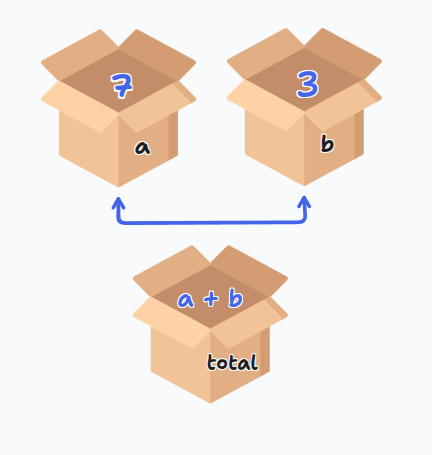
The = sign is for assignment, not mathematical equality. You're telling Python to store the right side value in the left side variable.
Multiple assignment:
x, y, z = 1, 2, 3
Variable Naming Rules
- Must start with letter or underscore
- Can contain letters, numbers, underscores
- Cannot start with number
- Cannot contain spaces
- Cannot use Python keywords (
for,if,class, etc.) - Case sensitive:
age,Age,AGEare different
Assignment Operators
x += 3 → Same as x = x + 3
x -= 2 → Same as x = x - 2
x *= 4 → Same as x = x * 4
x /= 2 → Same as x = x / 2
Reading Input
name = input("What's your name? ")
print(f"Hello, {name}!")
input() always returns a string! Even if the user types 42, you get "42".
Converting input:
age = int(input("How old are you? "))
price = float(input("Enter price: $"))
Practice
Ask for a number, print its square in a complete sentence ending with a period (use sep)
Compute: (512 - 282) / (47 × 48 + 5)
Convert kilograms to pounds (2.2 pounds per kilogram)
Basic Data Types
Strings
Text inside quotes:
name = "Mahmoud"
message = 'Hello'
Can use single or double quotes. Strings can contain letters, numbers, spaces, symbols.
Numbers
- int → Whole numbers:
7,0,-100 - float → Decimals:
3.14,0.5,-2.7
Boolean
True or false values:
print(5 > 3)        # True
print(2 == 10)      # False
print("a" in "cat") # True
Logical Operators
and → Both must be true
or → At least one must be true
not → Reverses the boolean
== → Equal to
!= → Not equal to
>, <, >=, <= → Comparisons
Practice
Read a DNA sequence and check:
1. Contains BOTH "A" AND "T"
2. Contains "U" OR "T"
3. Is pure RNA (no "T")
4. Is empty or only whitespace
5. Is valid DNA (only A, T, G, C)
6. Contains "A" OR "G" but NOT both
7. Contains any stop codon ("TAA", "TAG", "TGA")
Type Checking and Casting
print(type("hello"))  # <class 'str'>
print(type(10))       # <class 'int'>
print(type(3.5))      # <class 'float'>
print(type(True))     # <class 'bool'>
Type casting:
int("10")      # 10
float(5)       # 5.0
str(3.14)      # "3.14"
bool(0)        # False
bool(5)        # True
list("hi")     # ['h', 'i']
int("hello") and float("abc") will cause errors!
Sequences
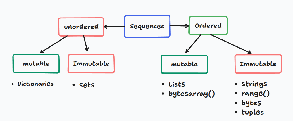
Strings
Strings are sequences of characters.
Indexing
Indexes start from 0:
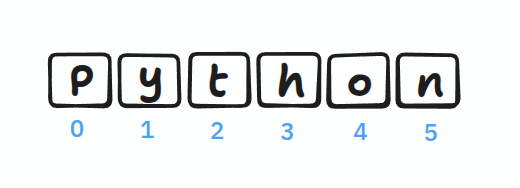
name = "Python"
print(name[0])   # P
print(name[3])   # h
You cannot change characters directly: name[0] = "J" causes an error!
But you can reassign the whole string: name = "Java"
String Operations
# Concatenation
"Hello" + " " + "World"  # "Hello World"

# Multiplication
"ha" * 3                 # "hahaha"

# Length
len("Python")            # 6

# Methods
text = "hello"
text.upper()             # "HELLO"
text.replace("h", "j")   # "jello"
Common String Methods
.upper(), .lower(), .capitalize(), .title()
.strip(), .lstrip(), .rstrip()
.replace(old, new), .split(sep), .join(list)
.find(sub), .count(sub)
.startswith(), .endswith()
.isalpha(), .isdigit(), .isalnum()
Practice
Convert DNA → RNA only if T exists (don't use if)
Check if DNA starts with "ATG" AND ends with "TAA"
Read text and print the last character
Lists
Lists can contain different types and are mutable (changeable).
numbers = [1, 2, 3]
mixed = [1, "hello", True]
List Operations
# Accessing
colors = ["red", "blue", "green"]
print(colors[1])  # "blue"

# Modifying (lists ARE mutable!)
colors[1] = "yellow"

# Adding
colors.append("black")          # Add at end
colors.insert(1, "white")       # Add at position

# Removing
del colors[1]                   # Remove by index
value = colors.pop()            # Remove last
colors.remove("red")            # Remove by value

# Sorting
numbers = [3, 1, 2]
numbers.sort()                  # Permanent
sorted(numbers)                 # Temporary

# Other operations
numbers.reverse()               # Reverse in place
len(numbers)                    # Length
Practice
Print the middle element of a list
Mutate RNA: ["A", "U", "G", "C", "U", "A"]
- Change first "A" to "G"
- Change last "A" to "C"
Swap first and last codon in: ["A","U","G","C","G","A","U","U","G"]
Create complementary DNA: A↔T, G↔C for ["A","T","G","C"]
Slicing
Extract portions of sequences: [start:stop:step]

[0:3] gives indices 0, 1, 2 (NOT 3)
Basic Slicing
numbers = [0, 1, 2, 3, 4, 5, 6, 7, 8, 9]

numbers[2:5]      # [2, 3, 4]
numbers[:3]       # [0, 1, 2] - from beginning
numbers[5:]       # [5, 6, 7, 8, 9] - to end
numbers[:]        # Copy everything
numbers[::2]      # [0, 2, 4, 6, 8] - every 2nd element
Negative Indices
Count from the end: -1 is last, -2 is second-to-last
numbers[-1]       # 9 - last element
numbers[-3:]      # [7, 8, 9] - last 3 elements
numbers[:-2]      # [0, 1, 2, 3, 4, 5, 6, 7] - all except last 2
numbers[::-1]     # Reverse!
Practice
Reverse middle 6 elements (indices 2-7) of [0,1,2,3,4,5,6,7,8,9]
Get every 3rd element backwards from ['a','b',...,'j']
Swap first 3 and last 3 characters in "abcdefghij"
Control Flow
If Statements
age = 18

if age >= 18:
    print("Adult")
elif age >= 13:
    print("Teen")
else:
    print("Child")
elif stops checking after first match. Separate if statements check all conditions.
Practice
Convert cm to inches (2.54 cm/inch). Print "invalid" if negative.
Print student year: ≤23: freshman, 24-53: sophomore, 54-83: junior, ≥84: senior
Number guessing game (1-10)
Loops
For Loops
# Loop through list
for fruit in ["apple", "banana"]:
    print(fruit)

# With index
for i, fruit in enumerate(["apple", "banana"]):
    print(f"{i}: {fruit}")

# Range
for i in range(5):        # 0, 1, 2, 3, 4
    print(i)

for i in range(2, 5):     # 2, 3, 4
    print(i)

for i in range(0, 10, 2): # 0, 2, 4, 6, 8
    print(i)
While Loops
count = 0
while count < 5:
    print(count)
    count += 1
Make sure your condition eventually becomes False!
Control Statements
break → Exit loop immediately
continue → Skip to next iteration
pass → Do nothing (placeholder)
Practice
Print your name 100 times
Print numbers and their squares from 1-20
Print: 8, 11, 14, 17, ..., 89 using a for loop
String & List Exercises
1. Count spaces to estimate words
2. Check if parentheses are balanced
3. Check if word contains vowels
4. Encrypt by rearranging even/odd indices
5. Capitalize first letter of each word
1. Replace all values > 10 with 10
2. Remove duplicates from list
3. Find longest run of zeros
4. Create [1,1,0,1,0,0,1,0,0,0,...]
5. Remove first character from each string
F-Strings (String Formatting)
Modern, clean way to format strings:
name = 'Ahmed'
age = 45
txt = f"My name is {name}, I am {age}"
Number Formatting
pi = 3.14159265359

f'{pi:.2f}'              # '3.14' - 2 decimals
f'{10:03d}'              # '010' - pad with zeros
f'{12345678:,d}'         # '12,345,678' - commas
f'{42:>10d}'             # '        42' - right align
f'{1234.5:>10,.2f}'      # '  1,234.50' - combined
Functions in F-Strings
name = "alice"
f"Hello, {name.upper()}!"        # 'Hello, ALICE!'

numbers = [3, 1, 4]
f"Sum: {sum(numbers)}"           # 'Sum: 8'
String Methods
split() and join()
# Split
text = "one,two,three"
words = text.split(',')          # ['one', 'two', 'three']
text.split()                     # Split on any whitespace

# Join
words = ['one', 'two', 'three']
', '.join(words)                 # 'one, two, three'
''.join(['H','e','l','l','o'])   # 'Hello'
partition()
Splits at first occurrence:
email = "user@example.com"
username, _, domain = email.partition('@')
# username = 'user', domain = 'example.com'
Character Checks
'123'.isdigit()          # True - all digits
'Hello123'.isalnum()     # True - letters and numbers
'hello'.isalpha()        # True - only letters
'hello'.islower()        # True - all lowercase
'HELLO'.isupper()        # True - all uppercase
Two Sum Problem
Given an array of integers and a target, return indices of two numbers that add up to target.
# Input: nums = [2, 7, 11, 15], target = 9
# Output: [0, 1]  (because 2 + 7 = 9)
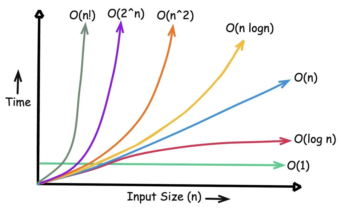
Brute Force Solution (O(n²))
nums = [2, 7, 11, 15]
target = 9

for i in range(len(nums)):
    for j in range(i + 1, len(nums)):
        if nums[i] + nums[j] == target:
            print([i, j])
Time complexity: O(n²)
10 elements = ~100 operations
1,000 elements = ~1,000,000 operations!
Unpacking with * and **
Unpacking Iterables (*)
# Basic unpacking
numbers = [1, 2, 3]
a, b, c = numbers

# Catch remaining items
first, *middle, last = [1, 2, 3, 4, 5]
# first = 1, middle = [2, 3, 4], last = 5

# In function calls
def add(a, b, c):
    return a + b + c

numbers = [1, 2, 3]
add(*numbers)  # Same as add(1, 2, 3)

# Combining lists
list1 = [1, 2]
list2 = [3, 4]
combined = [*list1, *list2]  # [1, 2, 3, 4]
Unpacking Dictionaries (**)
# Merge dictionaries
defaults = {'color': 'blue', 'size': 'M'}
custom = {'size': 'L'}
final = {**defaults, **custom}
# {'color': 'blue', 'size': 'L'}

# In function calls
def create_user(name, age, city):
    print(f"{name}, {age}, {city}")

data = {'name': 'Bob', 'age': 30, 'city': 'NYC'}
create_user(**data)
* unpacks iterables into positional arguments
** unpacks dictionaries into keyword arguments
Functions
A function is a reusable block of code that performs a specific task. It's like a recipe you can follow multiple times without rewriting the steps.
The DRY Principle
If you're copying and pasting code, you should probably write a function instead!
Without a function (repetitive):
# Calculating area three times - notice the pattern?
area1 = 10 * 5
print(f"Area 1: {area1}")

area2 = 8 * 6
print(f"Area 2: {area2}")

area3 = 12 * 4
print(f"Area 3: {area3}")
With a function (clean):
def calculate_area(length, width):
    return length * width

print(f"Area 1: {calculate_area(10, 5)}")
print(f"Area 2: {calculate_area(8, 6)}")
print(f"Area 3: {calculate_area(12, 4)}")
Basic Function Syntax
Declaring a Function
def greet():
    print("Hello, World!")
Anatomy:
def→ keyword to start a functiongreet→ function name (use descriptive names!)()→ parentheses for parameters:→ colon to start the body- Indented code → what the function does
Calling a Function
Defining a function doesn't run it! You must call it.
def greet():
    print("Hello, World!")

greet()  # Now it runs!
greet()  # You can call it multiple times
Parameters and Arguments
Parameters are in the definition. Arguments are the actual values you pass.
def greet(name):      # 'name' is a parameter
    print(f"Hello, {name}!")

greet("Alice")        # "Alice" is an argument
Multiple parameters:
def add_numbers(a, b):
    result = a + b
    print(f"{a} + {b} = {result}")

add_numbers(5, 3)     # Output: 5 + 3 = 8
Return Values
Functions can give back results using return:
def multiply(a, b):
    return a * b

result = multiply(4, 5)
print(result)  # 20

# Use the result directly in calculations
total = multiply(3, 7) + multiply(2, 4)  # 21 + 8 = 29
print() shows output on screen. return sends a value back so you can use it later.
Default Arguments
Give parameters default values if no argument is provided:
def power(base, exponent=2):  # exponent defaults to 2
    return base ** exponent

print(power(5))      # 25 (5²)
print(power(5, 3))   # 125 (5³)
Multiple defaults:
def create_profile(name, age=18, country="USA"):
    print(f"{name}, {age} years old, from {country}")

create_profile("Alice")                    # Uses both defaults
create_profile("Bob", 25)                  # Uses country default
create_profile("Charlie", 30, "Canada")    # No defaults used
Parameters with defaults must come after parameters without defaults!
# ❌ Wrong
def bad(a=5, b):
    pass

# ✅ Correct
def good(b, a=5):
    pass
Variable Number of Arguments
*args (Positional Arguments)
Use when you don't know how many arguments will be passed:
def sum_all(*numbers):
    total = 0
    for num in numbers:
        total += num
    return total

print(sum_all(1, 2, 3))           # 6
print(sum_all(10, 20, 30, 40))    # 100
**kwargs (Keyword Arguments)
Use for named arguments as a dictionary:
def print_info(**details):
    for key, value in details.items():
        print(f"{key}: {value}")

print_info(name="Alice", age=25, city="New York")
# Output:
# name: Alice
# age: 25
# city: New York
Combining Everything
When combining, use this order: regular params → *args → default params → **kwargs
def flexible(required, *args, default="default", **kwargs):
    print(f"Required: {required}")
    print(f"Args: {args}")
    print(f"Default: {default}")
    print(f"Kwargs: {kwargs}")

flexible("Must have", 1, 2, 3, default="Custom", extra="value")
Scope: Local vs Global
Scope determines where a variable can be accessed in your code.
Local scope: Variables inside functions only exist inside that function
def calculate():
    result = 10 * 5  # Local variable
    print(result)

calculate()        # 50
print(result)      # ❌ ERROR! result doesn't exist here
Global scope: Variables outside functions can be accessed anywhere
total = 0  # Global variable

def add_to_total(amount):
    global total  # Modify the global variable
    total += amount

add_to_total(10)
print(total)  # 10
Avoid global variables! Pass values as arguments and return results instead.
Better approach:
def add_to_total(current, amount):
    return current + amount

total = 0
total = add_to_total(total, 10)  # 10
total = add_to_total(total, 5)   # 15
Decomposition
Breaking complex problems into smaller, manageable functions. Each function should do one thing well.
Bad (one giant function):
def process_order(items, customer):
    # Calculate, discount, tax, print - all in one!
    total = sum(item['price'] for item in items)
    if total > 100:
        total *= 0.9
    total *= 1.08
    print(f"Customer: {customer}")
    print(f"Total: ${total:.2f}")
Good (decomposed):
def calculate_subtotal(items):
    return sum(item['price'] for item in items)

def apply_discount(amount):
    return amount * 0.9 if amount > 100 else amount

def add_tax(amount):
    return amount * 1.08

def print_receipt(customer, total):
    print(f"Customer: {customer}")
    print(f"Total: ${total:.2f}")

def process_order(items, customer):
    subtotal = calculate_subtotal(items)
    discounted = apply_discount(subtotal)
    final = add_tax(discounted)
    print_receipt(customer, final)
Benefits: ✅ Easier to understand ✅ Easier to test ✅ Reusable components ✅ Easier to debug
Practice Exercises
Write a function rectangle(m, n) that prints an m × n box of asterisks.
rectangle(2, 4)
# Output:
# ****
# ****
Write add_excitement(words) that adds "!" to each string in a list.
- Version A: Modify the original list
- Version B: Return a new list without modifying the original
words = ["hello", "world"]
add_excitement(words)
# words is now ["hello!", "world!"]
Write sum_digits(num) that returns the sum of all digits in a number.
sum_digits(123)   # Returns: 6 (1 + 2 + 3)
sum_digits(4567)  # Returns: 22 (4 + 5 + 6 + 7)
Write first_diff(str1, str2) that returns the first position where strings differ, or -1 if identical.
first_diff("hello", "world")  # Returns: 0
first_diff("test", "tent")    # Returns: 2
first_diff("same", "same")    # Returns: -1
A 3×3 board uses: 0 = empty, 1 = X, 2 = O
- Part A: Write a function that randomly places a 2 in an empty spot
- Part B: Write a function that checks if someone has won (returns True/False)
Write matches(str1, str2) that counts how many positions have the same character.
matches("python", "path") # Returns: 3 (positions 0, 2, 3)
Write findall(string, char) that returns a list of all positions where a character appears.
findall("hello", "l")  # Returns: [2, 3]
findall("test", "x")   # Returns: []
Write change_case(string) that swaps uppercase ↔ lowercase.
change_case("Hello World") # Returns: "hELLO wORLD"
Challenge Exercises
Write merge(list1, list2) that combines two sorted lists into one sorted list.
- Try it with
.sort()method - Try it without using
.sort()
merge([1, 3, 5], [2, 4, 6]) # Returns: [1, 2, 3, 4, 5, 6]
Write verbose(num) that converts numbers to English words (up to 10¹⁵).
verbose(123456)
# Returns: "one hundred twenty-three thousand, four hundred fifty-six"
Convert base 10 numbers to base 20 using letters A-T (A=0, B=1, ..., T=19).
base20(0)    # Returns: "A"
base20(20)   # Returns: "BA"
base20(39)   # Returns: "BT"
base20(400)  # Returns: "BAA"
Write closest(L, n) that returns the largest element in L that doesn't exceed n.
closest([1, 6, 3, 9, 11], 8)  # Returns: 6
closest([5, 10, 15, 20], 12)  # Returns: 10
Higher-Order Functions
Higher-Order Function: A function that either takes another function as a parameter OR returns a function as a result.
Why Do We Need Them?
Imagine you have a list of numbers and you want to:
- Keep only the even numbers
- Keep only numbers greater than 10
- Keep only numbers divisible by 3
You could write three different functions... or write ONE function that accepts different "rules" as parameters!
Separate what to do (iterate through a list) from how to decide (the specific rule)
Worked Example: Filtering Numbers
Step 1: The Problem
We have a list of numbers: [3, 8, 15, 4, 22, 7, 11]
We want to filter them based on different conditions.
Step 2: Without Higher-Order Functions (Repetitive)
# Filter for even numbers
def filter_even(numbers):
    result = []
    for num in numbers:
        if num % 2 == 0:
            result.append(num)
    return result

# Filter for numbers > 10
def filter_large(numbers):
    result = []
    for num in numbers:
        if num > 10:
            result.append(num)
    return result
Notice how we're repeating the same loop structure? Only the condition changes!
Step 3: With Higher-Order Function (Smart)
def filter_numbers(numbers, condition):
    """
    Filter numbers based on any condition function.

    numbers: list of numbers
    condition: a function that returns True/False
    """
    result = []
    for num in numbers:
        if condition(num):  # Call the function we received!
            result.append(num)
    return result
Now we have ONE function that can work with ANY condition!
Step 4: Define Simple Condition Functions
def is_even(n):
    return n % 2 == 0

def is_large(n):
    return n > 10

def is_small(n):
    return n < 10
Step 5: Use It!
numbers = [3, 8, 15, 4, 22, 7, 11]

print(filter_numbers(numbers, is_even))   # [8, 4, 22]
print(filter_numbers(numbers, is_large))  # [15, 22, 11]
print(filter_numbers(numbers, is_small))  # [3, 8, 4, 7]
We pass the function name WITHOUT parentheses: is_even not is_even()
Practice Exercises
Complete this function:
def filter_words(words, condition):
    # Your code here
    pass

def is_long(word):
    return len(word) > 5

def starts_with_a(word):
    return word.lower().startswith('a')

# Test it:
words = ["apple", "cat", "banana", "amazing", "dog"]
print(filter_words(words, is_long))         # Should print: ["banana", "amazing"]
print(filter_words(words, starts_with_a))   # Should print: ["apple", "amazing"]
Write a higher-order function that transforms numbers:
def transform_numbers(numbers, transformer):
    # Your code here: apply transformer to each number
    pass

def double(n):
    return n * 2

def square(n):
    return n ** 2

# Test it:
nums = [1, 2, 3, 4, 5]
print(transform_numbers(nums, double))   # Should print: [2, 4, 6, 8, 10]
print(transform_numbers(nums, square))   # Should print: [1, 4, 9, 16, 25]
Create a function that grades scores using different grading systems:
def apply_grading(scores, grade_function):
    # Your code here
    pass

def strict_grade(score):
    if score >= 90:
        return 'A'
    elif score >= 80:
        return 'B'
    else:
        return 'C'

def pass_fail(score):
    return 'Pass' if score >= 60 else 'Fail'

# Test it:
scores = [95, 75, 85, 55]
print(apply_grading(scores, strict_grade))  # Should print: ['A', 'C', 'B', 'C']
print(apply_grading(scores, pass_fail))     # Should print: ['Pass', 'Pass', 'Pass', 'Fail']
Conclusion
1. Functions can be passed as parameters (like any other value)
2. The higher-order function provides the structure (loop, collection)
3. The parameter function provides the specific behavior (condition, transformation)
4. This makes code more reusable and flexible
Python has built-in higher-order functions you'll use all the time:
• sorted(items, key=function)
• map(function, items)
• filter(function, items)
Challenge Exercise
Write a higher-order function validate_sequences(sequences, validator) that checks a list of DNA sequences using different validation rules.
Validation functions to create:
is_valid_dna(seq)- checks if sequence contains only A, C, G, Tis_long_enough(seq)- checks if sequence is at least 10 charactershas_start_codon(seq)- checks if sequence starts with "ATG"
sequences = ["ATGCGATCG", "ATGXYZ", "AT", "ATGCCCCCCCCCC"]

# Your solution should work like this:
print(validate_sequences(sequences, is_valid_dna))
# [True, False, True, True]

print(validate_sequences(sequences, is_long_enough))
# [False, False, False, True]
Tuples and Sets
Part 1: Tuples
What is a Tuple?
A tuple is essentially an immutable list. Once created, you cannot change its contents.
# List - mutable (can change)
L = [1, 2, 3]
L[0] = 100  # Works fine

# Tuple - immutable (cannot change)
t = (1, 2, 3)
t[0] = 100  # TypeError: 'tuple' object does not support item assignment
Creating Tuples
# With parentheses
t = (1, 2, 3)

# Without parentheses (comma makes it a tuple)
t = 1, 2, 3

# Single element tuple (comma is required!)
t = (1,)    # This is a tuple
t = (1)     # This is just an integer!

# Empty tuple
t = ()
t = tuple()

# From a list
t = tuple([1, 2, 3])

# From a string
t = tuple("hello")  # ('h', 'e', 'l', 'l', 'o')
Common mistake:
# This is NOT a tuple
x = (5)
print(type(x))  # <class 'int'>

# This IS a tuple
x = (5,)
print(type(x))  # <class 'tuple'>
Accessing Tuple Elements
t = ('a', 'b', 'c', 'd', 'e')

# Indexing (same as lists)
print(t[0])     # 'a'
print(t[-1])    # 'e'

# Slicing
print(t[1:3])   # ('b', 'c')
print(t[:3])    # ('a', 'b', 'c')
print(t[2:])    # ('c', 'd', 'e')

# Length
print(len(t))   # 5
Why Use Tuples?
1. Faster and Less Memory
Tuples are more efficient than lists:
import sys

L = [1, 2, 3, 4, 5]
t = (1, 2, 3, 4, 5)

print(sys.getsizeof(L))  # 104 bytes
print(sys.getsizeof(t))  # 80 bytes (smaller!)
2. Safe - Data Cannot Be Changed
When you want to ensure data stays constant:
# RGB color that shouldn't change
RED = (255, 0, 0)
# RED[0] = 200  # Error! Can't modify

# Coordinates
location = (40.7128, -74.0060)  # New York
3. Can Be Dictionary Keys
Lists cannot be dictionary keys, but tuples can:
# This works
locations = {
    (40.7128, -74.0060): "New York",
    (51.5074, -0.1278): "London"
}
print(locations[(40.7128, -74.0060)])  # New York

# This fails
# locations = {[40.7128, -74.0060]: "New York"}  # TypeError!
4. Return Multiple Values
Functions can return tuples:
def get_stats(numbers):
    return min(numbers), max(numbers), sum(numbers)

low, high, total = get_stats([1, 2, 3, 4, 5])
print(low, high, total)  # 1 5 15
Tuple Unpacking
# Basic unpacking
t = (1, 2, 3)
a, b, c = t
print(a, b, c)  # 1 2 3

# Swap values (elegant!)
x, y = 10, 20
x, y = y, x
print(x, y)  # 20 10

# Unpacking with *
t = (1, 2, 3, 4, 5)
first, *middle, last = t
print(first)   # 1
print(middle)  # [2, 3, 4]
print(last)    # 5
Looping Through Tuples
t = ('a', 'b', 'c')

# Basic loop
for item in t:
    print(item)

# With index
for i, item in enumerate(t):
    print(f"{i}: {item}")

# Loop through list of tuples
points = [(0, 0), (1, 2), (3, 4)]
for x, y in points:
    print(f"x={x}, y={y}")
Tuple Methods
Tuples have only two methods (because they're immutable):
t = (1, 2, 3, 2, 2, 4)

# Count occurrences
print(t.count(2))   # 3

# Find index
print(t.index(3))   # 2
Tuples vs Lists Summary
| Feature | Tuple | List |
|---|---|---|
| Syntax | (1, 2, 3) | [1, 2, 3] |
| Mutable | No | Yes |
| Speed | Faster | Slower |
| Memory | Less | More |
| Dictionary key | Yes | No |
| Use case | Fixed data | Changing data |
Tuple Exercises
Exercise 1: Create a tuple with your name, age, and city. Print each element.
Exercise 2: Given t = (1, 2, 3, 4, 5), print the first and last elements.
Exercise 3: Write a function that returns the min, max, and average of a list as a tuple.
Exercise 4: Swap two variables using tuple unpacking.
Exercise 5: Create a tuple from the string "ATGC" and count how many times 'A' appears.
Exercise 6: Given a list of (x, y) coordinates, calculate the distance of each from origin.
Exercise 7: Use a tuple as a dictionary key to store city names by their (latitude, longitude).
Exercise 8: Unpack (1, 2, 3, 4, 5) into first, middle (as list), and last.
Exercise 9: Create a function that returns the quotient and remainder of two numbers as a tuple.
Exercise 10: Loop through [(1, 'a'), (2, 'b'), (3, 'c')] and print each pair.
Exercise 11: Convert a list [1, 2, 3] to a tuple and back to a list.
Exercise 12: Find the index of 'G' in the tuple ('A', 'T', 'G', 'C').
Exercise 13: Create a tuple of tuples representing a 3x3 grid and print the center element.
Exercise 14: Given two tuples, concatenate them into a new tuple.
Exercise 15: Sort a list of (name, score) tuples by score in descending order.
Solutions
# Exercise 1
person = ("Mahmoud", 25, "Bologna")
print(person[0], person[1], person[2])

# Exercise 2
t = (1, 2, 3, 4, 5)
print(t[0], t[-1])

# Exercise 3
def stats(numbers):
    return min(numbers), max(numbers), sum(numbers)/len(numbers)
print(stats([1, 2, 3, 4, 5]))

# Exercise 4
x, y = 10, 20
x, y = y, x
print(x, y)

# Exercise 5
dna = tuple("ATGC")
print(dna.count('A'))

# Exercise 6
import math
coords = [(3, 4), (0, 5), (1, 1)]
for x, y in coords:
    dist = math.sqrt(x**2 + y**2)
    print(f"({x}, {y}): {dist:.2f}")

# Exercise 7
cities = {
    (40.71, -74.00): "New York",
    (51.51, -0.13): "London"
}
print(cities[(40.71, -74.00)])

# Exercise 8
t = (1, 2, 3, 4, 5)
first, *middle, last = t
print(first, middle, last)

# Exercise 9
def div_mod(a, b):
    return a // b, a % b
print(div_mod(17, 5))  # (3, 2)

# Exercise 10
pairs = [(1, 'a'), (2, 'b'), (3, 'c')]
for num, letter in pairs:
    print(f"{num}: {letter}")

# Exercise 11
L = [1, 2, 3]
t = tuple(L)
L2 = list(t)
print(t, L2)

# Exercise 12
dna = ('A', 'T', 'G', 'C')
print(dna.index('G'))  # 2

# Exercise 13
grid = ((1, 2, 3), (4, 5, 6), (7, 8, 9))
print(grid[1][1])  # 5

# Exercise 14
t1 = (1, 2)
t2 = (3, 4)
t3 = t1 + t2
print(t3)  # (1, 2, 3, 4)

# Exercise 15
scores = [("Alice", 85), ("Bob", 92), ("Charlie", 78)]
sorted_scores = sorted(scores, key=lambda x: x[1], reverse=True)
print(sorted_scores)
Part 2: Sets
What is a Set?
A set is a collection of unique elements with no duplicates. Sets work like mathematical sets.
# Duplicates are automatically removed
S = {1, 2, 2, 3, 3, 3}
print(S)  # {1, 2, 3}

# Unordered - no indexing
# print(S[0])  # TypeError!
Creating Sets
# With curly braces
S = {1, 2, 3, 4, 5}

# From a list (removes duplicates)
S = set([1, 2, 2, 3, 3])
print(S)  # {1, 2, 3}

# From a string
S = set("hello")
print(S)  # {'h', 'e', 'l', 'o'}  (no duplicate 'l')

# Empty set (NOT {} - that's an empty dict!)
S = set()
print(type(S))   # <class 'set'>
print(type({}))  # <class 'dict'>
Adding and Removing Elements
S = {1, 2, 3}

# Add single element
S.add(4)
print(S)  # {1, 2, 3, 4}

# Add multiple elements
S.update([5, 6, 7])
print(S)  # {1, 2, 3, 4, 5, 6, 7}

# Remove element (raises error if not found)
S.remove(7)
print(S)  # {1, 2, 3, 4, 5, 6}

# Discard element (no error if not found)
S.discard(100)  # No error
S.discard(6)
print(S)  # {1, 2, 3, 4, 5}

# Pop random element
x = S.pop()
print(x)  # Some element (unpredictable which one)

# Clear all elements
S.clear()
print(S)  # set()
Membership Testing
Very fast - O(1):
S = {1, 2, 3, 4, 5}

print(3 in S)     # True
print(100 in S)   # False
print(100 not in S)  # True
Looping Through Sets
S = {'a', 'b', 'c'}

# Basic loop
for item in S:
    print(item)

# With enumerate
for i, item in enumerate(S):
    print(f"{i}: {item}")
Note: Sets are unordered - iteration order is not guaranteed!
Set Operations (The Powerful Part!)
Sets support mathematical set operations.
Union: Elements in Either Set
A = {1, 2, 3}
B = {3, 4, 5}

# Using | operator
print(A | B)  # {1, 2, 3, 4, 5}

# Using method
print(A.union(B))  # {1, 2, 3, 4, 5}
Intersection: Elements in Both Sets
A = {1, 2, 3}
B = {3, 4, 5}

# Using & operator
print(A & B)  # {3}

# Using method
print(A.intersection(B))  # {3}
Difference: Elements in A but Not in B
A = {1, 2, 3}
B = {3, 4, 5}

# Using - operator
print(A - B)  # {1, 2}
print(B - A)  # {4, 5}

# Using method
print(A.difference(B))  # {1, 2}
Symmetric Difference: Elements in Either but Not Both
A = {1, 2, 3}
B = {3, 4, 5}

# Using ^ operator
print(A ^ B)  # {1, 2, 4, 5}

# Using method
print(A.symmetric_difference(B))  # {1, 2, 4, 5}
Subset and Superset
A = {1, 2}
B = {1, 2, 3, 4}

# Is A a subset of B?
print(A <= B)        # True
print(A.issubset(B)) # True

# Is B a superset of A?
print(B >= A)          # True
print(B.issuperset(A)) # True

# Proper subset (subset but not equal)
print(A < B)  # True
print(A < A)  # False
Disjoint: No Common Elements
A = {1, 2}
B = {3, 4}
C = {2, 3}

print(A.isdisjoint(B))  # True (no overlap)
print(A.isdisjoint(C))  # False (2 is common)
Set Operations Summary
| Operation | Operator | Method | Result |
|---|---|---|---|
| Union | A \| B | A.union(B) | All elements from both |
| Intersection | A & B | A.intersection(B) | Common elements |
| Difference | A - B | A.difference(B) | In A but not in B |
| Symmetric Diff | A ^ B | A.symmetric_difference(B) | In either but not both |
| Subset | A <= B | A.issubset(B) | True if A ⊆ B |
| Superset | A >= B | A.issuperset(B) | True if A ⊇ B |
| Disjoint | - | A.isdisjoint(B) | True if no overlap |
In-Place Operations
Modify the set directly (note the method names end in _update):
A = {1, 2, 3}
B = {3, 4, 5}

# Union in-place
A |= B  # or A.update(B)
print(A)  # {1, 2, 3, 4, 5}

# Intersection in-place
A = {1, 2, 3}
A &= B  # or A.intersection_update(B)
print(A)  # {3}

# Difference in-place
A = {1, 2, 3}
A -= B  # or A.difference_update(B)
print(A)  # {1, 2}
Practical Examples
Remove Duplicates from List
L = [1, 2, 2, 3, 3, 3, 4]
unique = list(set(L))
print(unique)  # [1, 2, 3, 4]
Find Common Elements
list1 = [1, 2, 3, 4]
list2 = [3, 4, 5, 6]
common = set(list1) & set(list2)
print(common)  # {3, 4}
Find Unique DNA Bases
dna = "ATGCATGCATGC"
bases = set(dna)
print(bases)  # {'A', 'T', 'G', 'C'}
Set Exercises
Exercise 1: Create a set from the list [1, 2, 2, 3, 3, 3] and print it.
Exercise 2: Add the number 10 to a set {1, 2, 3}.
Exercise 3: Remove duplicates from [1, 1, 2, 2, 3, 3, 4, 4].
Exercise 4: Find common elements between {1, 2, 3, 4} and {3, 4, 5, 6}.
Exercise 5: Find elements in {1, 2, 3} but not in {2, 3, 4}.
Exercise 6: Find all unique characters in the string "mississippi".
Exercise 7: Check if {1, 2} is a subset of {1, 2, 3, 4}.
Exercise 8: Find symmetric difference of {1, 2, 3} and {3, 4, 5}.
Exercise 9: Check if two sets {1, 2} and {3, 4} have no common elements.
Exercise 10: Given DNA sequence "ATGCATGC", create set of unique nucleotides.
Exercise 11: Combine sets {1, 2}, {3, 4}, {5, 6} into one set.
Exercise 12: Given two lists of students, find students in both classes.
Exercise 13: Remove element 3 from set {1, 2, 3, 4} safely (no error if missing).
Exercise 14: Create a set of prime numbers less than 20 and check membership of 17.
Exercise 15: Given three sets A, B, C, find elements that are in all three.
Solutions
# Exercise 1
S = set([1, 2, 2, 3, 3, 3])
print(S)  # {1, 2, 3}

# Exercise 2
S = {1, 2, 3}
S.add(10)
print(S)

# Exercise 3
L = [1, 1, 2, 2, 3, 3, 4, 4]
print(list(set(L)))

# Exercise 4
A = {1, 2, 3, 4}
B = {3, 4, 5, 6}
print(A & B)  # {3, 4}

# Exercise 5
A = {1, 2, 3}
B = {2, 3, 4}
print(A - B)  # {1}

# Exercise 6
print(set("mississippi"))

# Exercise 7
A = {1, 2}
B = {1, 2, 3, 4}
print(A <= B)  # True

# Exercise 8
A = {1, 2, 3}
B = {3, 4, 5}
print(A ^ B)  # {1, 2, 4, 5}

# Exercise 9
A = {1, 2}
B = {3, 4}
print(A.isdisjoint(B))  # True

# Exercise 10
dna = "ATGCATGC"
print(set(dna))  # {'A', 'T', 'G', 'C'}

# Exercise 11
A = {1, 2}
B = {3, 4}
C = {5, 6}
print(A | B | C)  # {1, 2, 3, 4, 5, 6}

# Exercise 12
class1 = ["Alice", "Bob", "Charlie"]
class2 = ["Bob", "Diana", "Charlie"]
print(set(class1) & set(class2))  # {'Bob', 'Charlie'}

# Exercise 13
S = {1, 2, 3, 4}
S.discard(3)  # Safe removal
S.discard(100)  # No error
print(S)

# Exercise 14
primes = {2, 3, 5, 7, 11, 13, 17, 19}
print(17 in primes)  # True

# Exercise 15
A = {1, 2, 3, 4}
B = {2, 3, 4, 5}
C = {3, 4, 5, 6}
print(A & B & C)  # {3, 4}
Summary: When to Use What?
| Data Type | Use When |
|---|---|
| List | Ordered, allow duplicates, need to modify |
| Tuple | Ordered, no modification needed, dictionary keys |
| Set | No duplicates, fast membership testing, set operations |
| Dict | Key-value mapping, fast lookup by key |
Useful modules
This is planned to be added later
Files and Sys Module
Reading Files
Files automatically close, even if errors occur. This is the modern, safe way.
# ✅ Best way - file automatically closes
with open("data.txt", "r") as file:
    content = file.read()
    print(content)

# ❌ Old way - must manually close (don't do this)
file = open("data.txt", "r")
content = file.read()
file.close()  # Easy to forget!
File Modes
"r" → Read (default)
"w" → Write (overwrites entire file!)
"a" → Append (adds to end)
"x" → Create (fails if exists)
"rb"/"wb" → Binary modes
# Read
with open("data.txt", "r") as f:
    content = f.read()

# Write (overwrites!)
with open("output.txt", "w") as f:
    f.write("Hello, World!")

# Append (adds to end)
with open("log.txt", "a") as f:
    f.write("New entry\n")
Reading Methods
read() - Entire File
with open("data.txt") as f:
    content = f.read()  # Whole file as string
readline() - One Line at a Time
with open("data.txt") as f:
    first = f.readline()   # First line
    second = f.readline()  # Second line
readlines() - All Lines as List
with open("data.txt") as f:
    lines = f.readlines()  # ['line1\n', 'line2\n', ...]
Looping Through Files
Most memory efficient - reads one line at a time. Works with huge files!
# Best way - memory efficient
with open("data.txt") as f:
    for line in f:
        print(line, end="")  # Line already has \n

# With line numbers
with open("data.txt") as f:
    for i, line in enumerate(f, start=1):
        print(f"{i}: {line}", end="")

# Strip newlines
with open("data.txt") as f:
    for line in f:
        line = line.strip()  # Remove \n
        print(line)

# Process as list
with open("data.txt") as f:
    lines = [line.strip() for line in f]
Writing Files
write() - Single String
with open("output.txt", "w") as f:
    f.write("Hello\n")
    f.write("World\n")
writelines() - List of Strings
You must include \n yourself!
lines = ["Line 1\n", "Line 2\n", "Line 3\n"]
with open("output.txt", "w") as f:
    f.writelines(lines)
print() to File
with open("output.txt", "w") as f:
    print("Hello, World!", file=f)
    print("Another line", file=f)
Processing Lines
Splitting
# By delimiter
line = "name,age,city"
parts = line.split(",")  # ['name', 'age', 'city']

# By whitespace (default)
line = "John   25   NYC"
parts = line.split()  # ['John', '25', 'NYC']

# With max splits
line = "a,b,c,d,e"
parts = line.split(",", 2)  # ['a', 'b', 'c,d,e']
Joining
words = ['Hello', 'World']
sentence = " ".join(words)  # "Hello World"

lines = ['line1', 'line2', 'line3']
content = "\n".join(lines)
Processing CSV Data
with open("data.csv") as f:
    for line in f:
        parts = line.strip().split(",")
        name, age, city = parts
        print(f"{name} is {age} from {city}")
The sys Module
Command Line Arguments
import sys

print(sys.argv)  # List of all arguments
# python script.py hello world
# Output: ['script.py', 'hello', 'world']

print(sys.argv[0])  # Script name
print(sys.argv[1])  # First argument
print(len(sys.argv))  # Number of arguments
Basic Argument Handling
import sys

if len(sys.argv) < 2:
    print("Usage: python script.py <filename>")
    sys.exit(1)

filename = sys.argv[1]
print(f"Processing: {filename}")
Processing Multiple Arguments
import sys

# python script.py file1.txt file2.txt file3.txt
for filename in sys.argv[1:]:  # Skip script name
    print(f"Processing: {filename}")
Argument Validation
Validation pattern for command-line scripts
import sys
import os
def main():
# Check argument count
if len(sys.argv) != 3:
print("Usage: python script.py <input> <output>")
sys.exit(1)
input_file = sys.argv[1]
output_file = sys.argv[2]
# Check if input exists
if not os.path.exists(input_file):
print(f"Error: {input_file} not found")
sys.exit(1)
# Check if output exists
if os.path.exists(output_file):
response = input(f"{output_file} exists. Overwrite? (y/n): ")
if response.lower() != 'y':
print("Aborted")
sys.exit(0)
# Process files
process(input_file, output_file)
if __name__ == "__main__":
main()
Standard Streams
stdin, stdout, stderr
import sys
# Read from stdin
line = sys.stdin.readline()
# Write to stdout (like print)
sys.stdout.write("Hello\n")
# Write to stderr (for errors)
sys.stderr.write("Error: failed\n")
Reading from Pipe
# In terminal
cat data.txt | python script.py
echo "Hello" | python script.py
# script.py
import sys
for line in sys.stdin:
print(f"Received: {line.strip()}")
Exit Codes
0 → Success
1 → General error
2 → Command line error
import sys
# Exit with success
sys.exit(0)
# Exit with error
sys.exit(1)
# Exit with message
sys.exit("Error: something went wrong")
Useful sys Attributes
import sys
# Python version
print(sys.version) # '3.10.0 (default, ...)'
print(sys.version_info) # sys.version_info(major=3, ...)
# Platform
print(sys.platform) # 'linux', 'darwin', 'win32'
# Module search paths
print(sys.path)
# Maximum integer
print(sys.maxsize)
# Default encoding
print(sys.getdefaultencoding()) # 'utf-8'
Building Command Line Tools
Simple Script Template
#!/usr/bin/env python3
"""Simple command line tool."""
import sys
import os
def print_usage():
print("Usage: python tool.py <input_file>")
print("Options:")
print(" -h, --help Show help")
print(" -v, --verbose Verbose output")
def main():
# Parse arguments
if len(sys.argv) < 2 or sys.argv[1] in ['-h', '--help']:
print_usage()
sys.exit(0)
verbose = '-v' in sys.argv or '--verbose' in sys.argv
# Get input file
input_file = None
for arg in sys.argv[1:]:
if not arg.startswith('-'):
input_file = arg
break
if not input_file:
print("Error: No input file", file=sys.stderr)
sys.exit(1)
if not os.path.exists(input_file):
print(f"Error: {input_file} not found", file=sys.stderr)
sys.exit(1)
# Process
if verbose:
print(f"Processing {input_file}...")
with open(input_file) as f:
for line in f:
print(line.strip())
if verbose:
print("Done!")
if __name__ == "__main__":
main()
Word Count Tool
Count lines, words, and characters
#!/usr/bin/env python3
import sys
def count_file(filename):
lines = words = chars = 0
with open(filename) as f:
for line in f:
lines += 1
words += len(line.split())
chars += len(line)
return lines, words, chars
def main():
if len(sys.argv) < 2:
print("Usage: python wc.py <file1> [file2] ...")
sys.exit(1)
total_l = total_w = total_c = 0
for filename in sys.argv[1:]:
try:
l, w, c = count_file(filename)
print(f"{l:8} {w:8} {c:8} {filename}")
total_l += l
total_w += w
total_c += c
except FileNotFoundError:
print(f"Error: {filename} not found", file=sys.stderr)
if len(sys.argv) > 2:
print(f"{total_l:8} {total_w:8} {total_c:8} total")
if __name__ == "__main__":
main()
FASTA Sequence Counter
#!/usr/bin/env python3
import sys
def process_fasta(filename):
sequences = 0
total_bases = 0
with open(filename) as f:
for line in f:
line = line.strip()
if line.startswith(">"):
sequences += 1
else:
total_bases += len(line)
return sequences, total_bases
def main():
if len(sys.argv) != 2:
print("Usage: python fasta_count.py <file.fasta>")
sys.exit(1)
filename = sys.argv[1]
try:
seqs, bases = process_fasta(filename)
print(f"Sequences: {seqs}")
print(f"Total bases: {bases}")
print(f"Average: {bases/seqs:.1f}")
except FileNotFoundError:
print(f"Error: {filename} not found", file=sys.stderr)
sys.exit(1)
if __name__ == "__main__":
main()
File Path Operations
import os
# Join paths (cross-platform)
path = os.path.join("folder", "subfolder", "file.txt")
# Get filename
os.path.basename("/path/to/file.txt") # "file.txt"
# Get directory
os.path.dirname("/path/to/file.txt") # "/path/to"
# Split extension
name, ext = os.path.splitext("data.txt") # "data", ".txt"
# Check existence
os.path.exists("file.txt") # True/False
os.path.isfile("file.txt") # True if file
os.path.isdir("folder") # True if directory
# Get file size
os.path.getsize("file.txt") # Size in bytes
# Get absolute path
os.path.abspath("file.txt")
Practice Exercises
1. Read file and print with line numbers
2. Count lines in a file
3. Copy file contents (use sys.argv)
4. Parse and format CSV rows
5. Reverse file contents
6. Search for word and print matching lines
7. Read stdin, write stdout in uppercase
8. Validate arguments (file must exist)
9. Word frequency counter (top 10 words)
10. Parse FASTA (extract names and lengths)
11. Merge multiple files into one
12. Remove blank lines from file
13. Convert file to uppercase
14. Log analyzer (count ERROR/WARNING/INFO)
15. Build grep-like tool: python grep.py <pattern> <file>
Quick Reference
with open(file) as f: → Open safely
f.read() → Read all
for line in f: → Iterate lines
f.write(string) → Write
sys.argv → Get arguments
sys.exit(code) → Exit program
print(..., file=sys.stderr) → Error output
os.path.exists(file) → Check file
os.path.join(a, b) → Join paths
Best Practices
1. Always use with for files
2. Validate command line arguments
3. Handle missing files gracefully
4. Use sys.exit(1) for errors
5. Write errors to stderr
6. Use os.path for cross-platform paths
Solution Hints
Use enumerate(f, start=1) when iterating
Check if word in line: for each line
Use from collections import Counter and .most_common(10)
Use re.search(pattern, line) for pattern matching
Recursive Functions
When a function calls itself to solve smaller versions of the same problem.
Classic example: Factorial (5! = 5 × 4 × 3 × 2 × 1)
def factorial(n):
# Base case: stop condition
if n == 0 or n == 1:
return 1
# Recursive case: call itself
return n * factorial(n - 1)
print(factorial(5)) # 120
How it works:
factorial(5) = 5 × factorial(4)
= 5 × (4 × factorial(3))
= 5 × (4 × (3 × factorial(2)))
= 5 × (4 × (3 × (2 × factorial(1))))
= 5 × (4 × (3 × (2 × 1)))
= 120
Key parts of recursion:
1. Base case: When to stop
2. Recursive case: Call itself with simpler input
3. Progress: Each call must get closer to the base case
Another example: Countdown
def countdown(n):
if n == 0:
print("Blast off!")
return
print(n)
countdown(n - 1)
countdown(3)
# Output: 3, 2, 1, Blast off!
Deep recursion can cause memory issues. Python has a default recursion limit.
Python Exceptions
Errors vs Bugs vs Exceptions
Syntax Errors
Errors in your code before it runs. Python can't even understand what you wrote.
# Missing colon
if True
print("Hello") # SyntaxError: expected ':'
# Unclosed parenthesis
print("Hello" # SyntaxError: '(' was never closed
Fix: Correct the syntax. Python tells you exactly where the problem is.
Bugs
Your code runs, but it does the wrong thing. No error message - just incorrect behavior.
# Bug: wrong formula
def circle_area(radius):
return 2 * 3.14 * radius # Wrong! This is circumference, not area
print(circle_area(5)) # Returns 31.4, should be 78.5
Why "bug"? Legend says early computers had actual insects causing problems. The term stuck.
Fix: Debug your code - find and fix the logic error.
Exceptions
Errors that occur during execution. The code is syntactically correct, but something goes wrong at runtime.
# Runs fine until...
x = 10 / 0 # ZeroDivisionError: division by zero
# Or...
my_list = [1, 2, 3]
print(my_list[10]) # IndexError: list index out of range
Fix: Handle the exception or prevent the error condition.
What is an Exception?
An exception is Python's way of saying "something unexpected happened and I can't continue."
When an exception occurs:
- Python stops normal execution
- Creates an exception object with error details
- Looks for code to handle it
- If no handler found, program crashes with traceback
# Exception in action
print("Start")
x = 10 / 0 # Exception here!
print("End") # Never reached
# Output:
# Start
# Traceback (most recent call last):
# File "example.py", line 2, in <module>
# x = 10 / 0
# ZeroDivisionError: division by zero
Common Exceptions
# ZeroDivisionError
10 / 0
# TypeError - wrong type
"hello" + 5
# ValueError - right type, wrong value
int("hello")
# IndexError - list index out of range
[1, 2, 3][10]
# KeyError - dictionary key not found
{'a': 1}['b']
# FileNotFoundError
open("nonexistent.txt")
# AttributeError - object has no attribute
"hello".append("!")
# NameError - variable not defined
print(undefined_variable)
# ImportError - module not found
import nonexistent_module
Handling Exceptions
Basic try/except
try:
x = 10 / 0
except:
print("Something went wrong!")
# Output: Something went wrong!
Problem: This catches ALL exceptions - even ones you didn't expect. Not recommended.
Catching Specific Exceptions (Recommended)
try:
x = 10 / 0
except ZeroDivisionError:
print("Cannot divide by zero!")
# Output: Cannot divide by zero!
Catching Multiple Specific Exceptions
try:
value = int(input("Enter a number: "))
result = 10 / value
except ValueError:
print("That's not a valid number!")
except ZeroDivisionError:
print("Cannot divide by zero!")
Catching Multiple Exceptions Together
try:
# Some risky code
pass
except (ValueError, TypeError):
print("Value or Type error occurred!")
Getting Exception Details
try:
x = 10 / 0
except ZeroDivisionError as e:
print(f"Error: {e}")
print(f"Type: {type(e).__name__}")
# Output:
# Error: division by zero
# Type: ZeroDivisionError
The Complete try/except/else/finally
try:
# Code that might raise an exception
result = 10 / 2
except ZeroDivisionError:
# Runs if exception occurs
print("Cannot divide by zero!")
else:
# Runs if NO exception occurs
print(f"Result: {result}")
finally:
# ALWAYS runs, exception or not
print("Cleanup complete")
# Output:
# Result: 5.0
# Cleanup complete
When to Use Each Part
| Block | When It Runs | Use For |
|---|---|---|
try | Always attempts | Code that might fail |
except | If exception occurs | Handle the error |
else | If NO exception | Code that depends on try success |
finally | ALWAYS | Cleanup (close files, connections) |
finally is Guaranteed
def risky_function():
try:
return 10 / 0
except ZeroDivisionError:
return "Error!"
finally:
print("This ALWAYS prints!")
result = risky_function()
# Output: This ALWAYS prints!
# result = "Error!"
Best Practices
1. Be Specific - Don't Catch Everything
# BAD - catches everything, hides bugs
try:
do_something()
except:
pass
# GOOD - catches only what you expect
try:
do_something()
except ValueError:
handle_value_error()
2. Don't Silence Exceptions Without Reason
# BAD - silently ignores errors
try:
important_operation()
except Exception:
pass # What went wrong? We'll never know!
# GOOD - at least log it
try:
important_operation()
except Exception as e:
print(f"Error occurred: {e}")
# or use logging.error(e)
3. Use else for Code That Depends on try Success
# Less clear
try:
file = open("data.txt")
content = file.read()
process(content)
except FileNotFoundError:
print("File not found")
# More clear - separate "risky" from "safe" code
try:
file = open("data.txt")
except FileNotFoundError:
print("File not found")
else:
content = file.read()
process(content)
4. Use finally for Cleanup
file = None
try:
file = open("data.txt")
content = file.read()
except FileNotFoundError:
print("File not found")
finally:
if file:
file.close() # Always close, even if error
# Even better - use context manager
with open("data.txt") as file:
content = file.read() # Automatically closes!
5. Catch Exceptions at the Right Level
# Don't catch too early
def read_config():
# Let the caller handle missing file
with open("config.txt") as f:
return f.read()
# Catch at appropriate level
def main():
try:
config = read_config()
except FileNotFoundError:
print("Config file missing, using defaults")
config = get_defaults()
Raising Exceptions
Use raise to throw your own exceptions:
def divide(a, b):
if b == 0:
raise ValueError("Cannot divide by zero!")
return a / b
try:
result = divide(10, 0)
except ValueError as e:
print(e) # Cannot divide by zero!
Re-raising Exceptions
try:
risky_operation()
except ValueError:
print("Logging this error...")
raise # Re-raise the same exception
Built-in Exception Hierarchy
All exceptions inherit from BaseException. Here's the hierarchy:
BaseException
├── SystemExit
├── KeyboardInterrupt
├── GeneratorExit
└── Exception
├── StopIteration
├── ArithmeticError
│ ├── FloatingPointError
│ ├── OverflowError
│ └── ZeroDivisionError
├── AssertionError
├── AttributeError
├── BufferError
├── EOFError
├── ImportError
│ └── ModuleNotFoundError
├── LookupError
│ ├── IndexError
│ └── KeyError
├── MemoryError
├── NameError
│ └── UnboundLocalError
├── OSError
│ ├── FileExistsError
│ ├── FileNotFoundError
│ ├── IsADirectoryError
│ ├── NotADirectoryError
│ ├── PermissionError
│ └── TimeoutError
├── ReferenceError
├── RuntimeError
│ ├── NotImplementedError
│ └── RecursionError
├── SyntaxError
│ └── IndentationError
│ └── TabError
├── TypeError
└── ValueError
└── UnicodeError
├── UnicodeDecodeError
├── UnicodeEncodeError
└── UnicodeTranslateError
Why Hierarchy Matters
Catching a parent catches all children:
# Catches ZeroDivisionError, OverflowError, FloatingPointError
try:
result = 10 / 0
except ArithmeticError:
print("Math error!")
# Catches IndexError and KeyError
try:
my_list[100]
except LookupError:
print("Lookup failed!")
Tip: Catch Exception instead of bare except: - it doesn't catch KeyboardInterrupt or SystemExit.
# Better than bare except
try:
do_something()
except Exception as e:
print(f"Error: {e}")
User-Defined Exceptions
Create custom exceptions by inheriting from Exception:
Basic Custom Exception
class InvalidDNAError(Exception):
"""Raised when DNA sequence contains invalid characters"""
pass
def validate_dna(sequence):
valid_bases = set("ATGC")
for base in sequence.upper():
if base not in valid_bases:
raise InvalidDNAError(f"Invalid base: {base}")
return True
try:
validate_dna("ATGXCCC")
except InvalidDNAError as e:
print(f"Invalid DNA: {e}")
Custom Exception with Attributes
class InsufficientFundsError(Exception):
"""Raised when account has insufficient funds"""
def __init__(self, balance, amount):
self.balance = balance
self.amount = amount
self.shortage = amount - balance
super().__init__(
f"Cannot withdraw ${amount}. "
f"Balance: ${balance}. "
f"Short by: ${self.shortage}"
)
class BankAccount:
def __init__(self, balance):
self.balance = balance
def withdraw(self, amount):
if amount > self.balance:
raise InsufficientFundsError(self.balance, amount)
self.balance -= amount
return amount
# Usage
account = BankAccount(100)
try:
account.withdraw(150)
except InsufficientFundsError as e:
print(e)
print(f"You need ${e.shortage} more")
# Output:
# Cannot withdraw $150. Balance: $100. Short by: $50
# You need $50 more
Exception Hierarchy for Your Project
# Base exception for your application
class BioinformaticsError(Exception):
"""Base exception for bioinformatics operations"""
pass
# Specific exceptions
class SequenceError(BioinformaticsError):
"""Base for sequence-related errors"""
pass
class InvalidDNAError(SequenceError):
"""Invalid DNA sequence"""
pass
class InvalidRNAError(SequenceError):
"""Invalid RNA sequence"""
pass
class AlignmentError(BioinformaticsError):
"""Sequence alignment failed"""
pass
# Now you can catch at different levels
try:
process_sequence()
except InvalidDNAError:
print("DNA issue")
except SequenceError:
print("Some sequence issue")
except BioinformaticsError:
print("General bioinformatics error")
Exercises
Exercise 1: Write code that catches a ZeroDivisionError and prints a friendly message.
Exercise 2: Ask user for a number, handle both ValueError (not a number) and ZeroDivisionError (if dividing by it).
Exercise 3: Write a function that opens a file and handles FileNotFoundError.
Exercise 4: Create a function that takes a list and index, returns the element, handles IndexError.
Exercise 5: Write code that handles KeyError when accessing a dictionary.
Exercise 6: Create a custom NegativeNumberError and raise it if a number is negative.
Exercise 7: Write a function that converts string to int, handling ValueError, and returns 0 on failure.
Exercise 8: Use try/except/else/finally to read a file and ensure it's always closed.
Exercise 9: Create a custom InvalidAgeError with min and max age attributes.
Exercise 10: Write a function that validates an email (must contain @), raise ValueError if invalid.
Exercise 11: Handle multiple exceptions: TypeError, ValueError, ZeroDivisionError in one block.
Exercise 12: Create a hierarchy: ValidationError → EmailError, PhoneError.
Exercise 13: Re-raise an exception after logging it.
Exercise 14: Create a InvalidSequenceError for DNA validation with the invalid character as attribute.
Exercise 15: Write a "safe divide" function that returns None on any error instead of crashing.
Solutions
# Exercise 1
try:
result = 10 / 0
except ZeroDivisionError:
print("Cannot divide by zero!")
# Exercise 2
try:
num = int(input("Enter a number: "))
result = 100 / num
print(f"100 / {num} = {result}")
except ValueError:
print("That's not a valid number!")
except ZeroDivisionError:
print("Cannot divide by zero!")
# Exercise 3
def read_file(filename):
try:
with open(filename) as f:
return f.read()
except FileNotFoundError:
print(f"File '{filename}' not found")
return None
# Exercise 4
def safe_get(lst, index):
try:
return lst[index]
except IndexError:
print(f"Index {index} out of range")
return None
# Exercise 5
d = {'a': 1, 'b': 2}
try:
value = d['c']
except KeyError:
print("Key not found!")
value = None
# Exercise 6
class NegativeNumberError(Exception):
pass
def check_positive(n):
if n < 0:
raise NegativeNumberError(f"{n} is negative!")
return n
# Exercise 7
def safe_int(s):
try:
return int(s)
except ValueError:
return 0
# Exercise 8
file = None
try:
file = open("data.txt")
content = file.read()
except FileNotFoundError:
print("File not found")
content = ""
else:
print("File read successfully")
finally:
if file:
file.close()
print("Cleanup done")
# Exercise 9
class InvalidAgeError(Exception):
def __init__(self, age, min_age=0, max_age=150):
self.age = age
self.min_age = min_age
self.max_age = max_age
super().__init__(f"Age {age} not in range [{min_age}, {max_age}]")
# Exercise 10
def validate_email(email):
if '@' not in email:
raise ValueError(f"Invalid email: {email} (missing @)")
return True
# Exercise 11
try:
# risky code
pass
except (TypeError, ValueError, ZeroDivisionError) as e:
print(f"Error: {e}")
# Exercise 12
class ValidationError(Exception):
pass
class EmailError(ValidationError):
pass
class PhoneError(ValidationError):
pass
# Exercise 13
try:
result = 10 / 0
except ZeroDivisionError:
print("Logging: Division by zero occurred")
raise
# Exercise 14
class InvalidSequenceError(Exception):
def __init__(self, sequence, invalid_char):
self.sequence = sequence
self.invalid_char = invalid_char
super().__init__(f"Invalid character '{invalid_char}' in sequence")
def validate_dna(seq):
for char in seq:
if char not in "ATGC":
raise InvalidSequenceError(seq, char)
return True
# Exercise 15
def safe_divide(a, b):
try:
return a / b
except Exception:
return None
print(safe_divide(10, 2)) # 5.0
print(safe_divide(10, 0)) # None
print(safe_divide("a", 2)) # None
Summary
| Concept | Description |
|---|---|
| Syntax Error | Code is malformed, won't run |
| Bug | Code runs but gives wrong result |
| Exception | Runtime error, can be handled |
| try/except | Catch and handle exceptions |
| else | Runs if no exception |
| finally | Always runs (cleanup) |
| raise | Throw an exception |
| Custom Exception | Inherit from Exception |
Best Practices:
- Catch specific exceptions, not bare
except: - Don't silence exceptions without reason
- Use
finallyfor cleanup - Create custom exceptions for your domain
- Build exception hierarchies for complex projects
Debugging
Theory
PyCharm Debug Tutorial
Using the IDLE Debugger
Python Dictionaries
What is a Dictionary?
A dictionary stores data as key-value pairs.
# Basic structure
student = {'name': 'Alex', 'age': 20, 'major': 'CS'}
# Access by key
print(student['name']) # Alex
print(student['age']) # 20
Creating Dictionaries
# Empty dictionary
empty = {}
# With initial values
person = {'name': 'Alex', 'age': 20}
# Using dict() constructor
person = dict(name='Alex', age=20)
Basic Operations
Adding and Modifying
student = {'name': 'Alex', 'age': 20}
# Add new key
student['major'] = 'CS'
print(student) # {'name': 'Alex', 'age': 20, 'major': 'CS'}
# Modify existing value
student['age'] = 21
print(student) # {'name': 'Alex', 'age': 21, 'major': 'CS'}
Deleting
student = {'name': 'Alex', 'age': 20, 'major': 'CS'}
# Delete specific key
del student['major']
print(student) # {'name': 'Alex', 'age': 20}
# Remove and return value
age = student.pop('age')
print(age) # 20
print(student) # {'name': 'Alex'}
Getting Values Safely
student = {'name': 'Alex', 'age': 20}
# Direct access - raises error if key missing
print(student['name']) # Alex
# print(student['grade']) # KeyError!
# Safe access with .get() - returns None if missing
print(student.get('name')) # Alex
print(student.get('grade')) # None
# Provide default value
print(student.get('grade', 'N/A')) # N/A
Useful Methods
student = {'name': 'Alex', 'age': 20, 'major': 'CS'}
# Get all keys
print(student.keys()) # dict_keys(['name', 'age', 'major'])
# Get all values
print(student.values()) # dict_values(['Alex', 20, 'CS'])
# Get all key-value pairs
print(student.items()) # dict_items([('name', 'Alex'), ('age', 20), ('major', 'CS')])
# Get length
print(len(student)) # 3
Membership Testing
Use in to check if a key exists (not value!):
student = {'name': 'Alex', 'age': 20}
# Check if key exists
print('name' in student) # True
print('grade' in student) # False
# Check if key does NOT exist
print('grade' not in student) # True
# To check values, use .values()
print('Alex' in student.values()) # True
print(20 in student.values()) # True
Important: Checking in on a dictionary is O(1) - instant! This is why dictionaries are so powerful.
Looping Through Dictionaries
Loop Over Keys (Default)
student = {'name': 'Alex', 'age': 20, 'major': 'CS'}
# Default: loops over keys
for key in student:
print(key)
# name
# age
# major
# Explicit (same result)
for key in student.keys():
print(key)
Loop Over Values
student = {'name': 'Alex', 'age': 20, 'major': 'CS'}
for value in student.values():
print(value)
# Alex
# 20
# CS
Loop Over Keys and Values Together
student = {'name': 'Alex', 'age': 20, 'major': 'CS'}
for key, value in student.items():
print(f"{key}: {value}")
# name: Alex
# age: 20
# major: CS
Loop With Index Using enumerate()
student = {'name': 'Alex', 'age': 20, 'major': 'CS'}
for index, key in enumerate(student):
print(f"{index}: {key} = {student[key]}")
# 0: name = Alex
# 1: age = 20
# 2: major = CS
# Or with items()
for index, (key, value) in enumerate(student.items()):
print(f"{index}: {key} = {value}")
Dictionary Order
Python 3.7+: Dictionaries maintain insertion order.
# Items stay in the order you add them
d = {}
d['first'] = 1
d['second'] = 2
d['third'] = 3
for key in d:
print(key)
# first
# second
# third (guaranteed order!)
Note: Before Python 3.7, dictionary order was not guaranteed. If you need to support older Python, don't rely on order.
Important: While keys maintain insertion order, this doesn't mean dictionaries are sorted. They just remember the order you added things.
# Not sorted - just insertion order
d = {'c': 3, 'a': 1, 'b': 2}
print(list(d.keys())) # ['c', 'a', 'b'] - insertion order, not alphabetical
Complex Values
Lists as Values
student = {
'name': 'Alex',
'courses': ['Math', 'Physics', 'CS']
}
# Access list items
print(student['courses'][0]) # Math
# Modify list
student['courses'].append('Biology')
print(student['courses']) # ['Math', 'Physics', 'CS', 'Biology']
Nested Dictionaries
students = {
1: {'name': 'Alex', 'age': 20},
2: {'name': 'Maria', 'age': 22},
3: {'name': 'Jordan', 'age': 21}
}
# Access nested values
print(students[1]['name']) # Alex
print(students[2]['age']) # 22
# Modify nested values
students[3]['age'] = 22
# Add new entry
students[4] = {'name': 'Casey', 'age': 19}
Why Dictionaries Are Fast: Hashing
Dictionaries use hashing to achieve O(1) lookup time.
How it works:
- When you add a key, Python computes a hash (a number) from the key
- This hash tells Python exactly where to store the value in memory
- When you look up the key, Python computes the same hash and goes directly to that location
Result: Looking up a key takes the same time whether your dictionary has 10 items or 10 million items.
# List: O(n) - must check each element
my_list = [2, 7, 11, 15]
if 7 in my_list: # Checks: 2? no. 7? yes! (2 checks)
print("Found")
# Dictionary: O(1) - instant lookup
my_dict = {2: 'a', 7: 'b', 11: 'c', 15: 'd'}
if 7 in my_dict: # Goes directly to location (1 check)
print("Found")
Practical Example: Two Sum Problem
Problem: Find two numbers that add up to a target.
Slow approach (nested loops - O(n²)):
nums = [2, 7, 11, 15]
target = 9
for i in range(len(nums)):
for j in range(i + 1, len(nums)):
if nums[i] + nums[j] == target:
print([i, j]) # [0, 1]
Fast approach (dictionary - O(n)):
nums = [2, 7, 11, 15]
target = 9
seen = {}
for i, num in enumerate(nums):
complement = target - num
if complement in seen:
print([seen[complement], i]) # [0, 1]
else:
seen[num] = i
Why it's faster:
- We loop once through the array
- For each number, we check if its complement exists (O(1) lookup)
- Total: O(n) instead of O(n²)
Trace through:
i=0, num=2: complement=7, not in seen, add {2: 0}
i=1, num=7: complement=2, IS in seen at index 0, return [0, 1]
Exercises
Exercise 1: Create a dictionary of 5 countries and their capitals. Print each country and its capital.
Exercise 2: Write a program that counts how many times each character appears in a string.
Exercise 3: Given a list of numbers, create a dictionary where keys are numbers and values are their squares.
Exercise 4: Create a program that stores product names and prices. Let the user look up prices by product name.
Exercise 5: Given a 5×5 list of numbers, count how many times each number appears and print the three most common.
Exercise 6: DNA pattern matching - given a list of DNA sequences and a pattern with wildcards (*), find matching sequences:
sequences = ['ATGCATGC', 'ATGGATGC', 'TTGCATGC']
pattern = 'ATG*ATGC' # * matches any character
# Should match: 'ATGCATGC', 'ATGGATGC'
Solutions
# Exercise 1
capitals = {'France': 'Paris', 'Japan': 'Tokyo', 'Italy': 'Rome',
'Egypt': 'Cairo', 'Brazil': 'Brasilia'}
for country, capital in capitals.items():
print(f"{country}: {capital}")
# Exercise 2
text = "hello world"
char_count = {}
for char in text:
char_count[char] = char_count.get(char, 0) + 1
print(char_count)
# Exercise 3
numbers = [1, 2, 3, 4, 5]
squares = {n: n**2 for n in numbers}
print(squares) # {1: 1, 2: 4, 3: 9, 4: 16, 5: 25}
# Exercise 4
products = {}
while True:
name = input("Product name (or 'done'): ")
if name == 'done':
break
price = float(input("Price: "))
products[name] = price
while True:
lookup = input("Look up product (or 'quit'): ")
if lookup == 'quit':
break
print(products.get(lookup, "Product not found"))
# Exercise 5
import random
grid = [[random.randint(1, 10) for _ in range(5)] for _ in range(5)]
counts = {}
for row in grid:
for num in row:
counts[num] = counts.get(num, 0) + 1
# Sort by count and get top 3
top3 = sorted(counts.items(), key=lambda x: x[1], reverse=True)[:3]
print("Top 3:", top3)
# Exercise 6
sequences = ['ATGCATGC', 'ATGGATGC', 'TTGCATGC']
pattern = 'ATG*ATGC'
for seq in sequences:
match = True
for i, char in enumerate(pattern):
if char != '*' and char != seq[i]:
match = False
break
if match:
print(f"Match: {seq}")
Summary
| Operation | Syntax | Time |
|---|---|---|
| Create | d = {'a': 1} | O(1) |
| Access | d['key'] | O(1) |
| Add/Modify | d['key'] = value | O(1) |
| Delete | del d['key'] | O(1) |
| Check key exists | 'key' in d | O(1) |
| Get all keys | d.keys() | O(1) |
| Get all values | d.values() | O(1) |
| Loop | for k in d | O(n) |
Key takeaways:
- Dictionaries are fast for lookups (O(1))
- Use
.get()for safe access with default values - Loop with
.items()to get both keys and values - Python 3.7+ maintains insertion order
- Perfect for counting, caching, and mapping data
Regular Expressions in Python
Regular expressions (regex) are powerful patterns used to search, match, and manipulate text. You can find patterns, not just exact text.

Examples:
- Find all email addresses in a document
- Validate phone numbers
- Extract gene IDs from biological data
- Find DNA/RNA sequence patterns
- Clean messy text data
Getting Started
Import the Module
import re
Write regex patterns with the r prefix: r"pattern"
Why Raw Strings Matter
# Normal string - \n becomes a newline
print("Hello\nWorld")
# Output:
# Hello
# World
# Raw string - \n stays as literal characters
print(r"Hello\nWorld")
# Output: Hello\nWorld
In regex, backslashes are special! Raw strings prevent confusion:
# ❌ Confusing without raw string
pattern = "\\d+"
# ✅ Clean with raw string
pattern = r"\d+"
Always write regex patterns as raw strings: r"pattern"
Level 1: Literal Matching
The simplest regex matches exact text.
import re
dna = "ATGCGATCG"
# Search for exact text "ATG"
if re.search(r"ATG", dna):
print("Found ATG!")
Your First Function: re.search()
Looks for a pattern anywhere in text. Returns a match object if found, None if not.
match = re.search(r"ATG", "ATGCCC")
if match:
print("Found:", match.group()) # Found: ATG
print("Position:", match.start()) # Position: 0
Regex is case-sensitive by default! "ATG" ≠ "atg"
Practice
Find which sequences contain "ATG": ["ATGCCC", "TTTAAA", "ATGATG"]
Check if "PYTHON" appears in: "I love PYTHON programming"
Level 2: The Dot . - Match Any Character
The dot . matches any single character (except newline).
# Find "A" + any character + "G"
dna = "ATGCGATCG"
matches = re.findall(r"A.G", dna)
print(matches) # ['ATG', 'ACG']
New Function: re.findall()
Finds all matches and returns them as a list.
text = "cat bat rat"
print(re.findall(r".at", text)) # ['cat', 'bat', 'rat']
Practice
Match "b.t" (b + any char + t) in: "bat bet bit bot but"
Find all 3-letter patterns starting with 'c' in: "cat cow cup car"
Level 3: Character Classes [ ]
Square brackets let you specify which characters to match.
# Match any nucleotide (A, T, G, or C)
dna = "ATGCXYZ"
nucleotides = re.findall(r"[ATGC]", dna)
print(nucleotides) # ['A', 'T', 'G', 'C']
Character Ranges
Use - for ranges:
re.findall(r"[0-9]", "Room 123") # ['1', '2', '3']
re.findall(r"[a-z]", "Hello") # ['e', 'l', 'l', 'o']
re.findall(r"[A-Z]", "Hello") # ['H']
re.findall(r"[A-Za-z]", "Hello123") # ['H', 'e', 'l', 'l', 'o']
Negation with ^
^ inside brackets means "NOT these characters":
# Match anything that's NOT a nucleotide
dna = "ATGC-X123"
non_nucleotides = re.findall(r"[^ATGC]", dna)
print(non_nucleotides) # ['-', 'X', '1', '2', '3']
Practice
Find all digits in: "Gene ID: ABC123"
Find all vowels in: "bioinformatics"
Find all NON-digits in: "Room123"
Level 4: Quantifiers - Repeating Patterns
Quantifiers specify how many times a pattern repeats.
* → 0 or more times
+ → 1 or more times
? → 0 or 1 time (optional)
{n} → Exactly n times
{n,m} → Between n and m times
Examples
# Find sequences of 2+ C's
dna = "ATGCCCAAAGGG"
print(re.findall(r"C+", dna)) # ['CCC']
print(re.findall(r"C{2,}", dna)) # ['CCC']
# Find all digit groups
text = "Call 123 or 4567"
print(re.findall(r"\d+", text)) # ['123', '4567']
# Optional minus sign
print(re.findall(r"-?\d+", "123 -456 789")) # ['123', '-456', '789']
Combining with Character Classes
# Find all 3-letter codons
dna = "ATGCCCAAATTT"
codons = re.findall(r"[ATGC]{3}", dna)
print(codons) # ['ATG', 'CCC', 'AAA', 'TTT']
Practice
Find sequences of exactly 3 A's in: "ATGCCCAAAGGGTTT"
Match "colou?r" (u is optional) in: "color colour"
Find all digit sequences in: "123 4567 89"
Level 5: Escaping Special Characters
Special characters like . * + ? [ ] ( ) have special meanings. To match them literally, escape with \.
# ❌ Wrong - dot matches ANY character
text = "file.txt and fileXtxt"
print(re.findall(r"file.txt", text)) # ['file.txt', 'fileXtxt']
# ✅ Correct - escaped dot matches only literal dot
print(re.findall(r"file\.txt", text)) # ['file.txt']
Common Examples
re.search(r"\$100", "$100") # Literal dollar sign
re.search(r"What\?", "What?") # Literal question mark
re.search(r"C\+\+", "C++") # Literal plus signs
re.search(r"\(test\)", "(test)") # Literal parentheses
Practice
Match "data.txt" (with literal dot) in: "File: data.txt"
Match "c++" in: "I code in c++ and python"
Level 6: Predefined Shortcuts
Python provides shortcuts for common character types.
\d → Any digit [0-9]
\D → Any non-digit
\w → Word character [A-Za-z0-9_]
\W → Non-word character
\s → Whitespace (space, tab, newline)
\S → Non-whitespace
Examples
# Find all digits
text = "Room 123, Floor 4"
print(re.findall(r"\d+", text)) # ['123', '4']
# Find all words
sentence = "DNA_seq-123 test"
print(re.findall(r"\w+", sentence)) # ['DNA_seq', '123', 'test']
# Split on whitespace
data = "ATG CCC\tAAA"
print(re.split(r"\s+", data)) # ['ATG', 'CCC', 'AAA']
Practice
Find all word characters in: "Hello-World"
Split on whitespace: "ATG CCC\tAAA"
Level 7: Anchors - Position Matching
Anchors match positions, not characters.
^ → Start of string
$ → End of string
\b → Word boundary
\B → Not a word boundary
Examples
dna = "ATGCCCATG"
# Match only at start
print(re.search(r"^ATG", dna)) # Matches!
print(re.search(r"^CCC", dna)) # None
# Match only at end
print(re.search(r"ATG$", dna)) # Matches!
print(re.search(r"CCC$", dna)) # None
# Word boundaries - whole words only
text = "The cat concatenated strings"
print(re.findall(r"\bcat\b", text)) # ['cat'] - only the word
print(re.findall(r"cat", text)) # ['cat', 'cat'] - both
Practice
Find sequences starting with "ATG": ["ATGCCC", "CCCATG", "TACATG"]
Match whole word "cat" (not "concatenate") in: "The cat sat"
Level 8: Alternation - OR Operator |
The pipe | means "match this OR that".
# Match either ATG or AUG
dna = "ATG is DNA, AUG is RNA"
print(re.findall(r"ATG|AUG", dna)) # ['ATG', 'AUG']
# Match stop codons
rna = "AUGCCCUAAUAGUGA"
print(re.findall(r"UAA|UAG|UGA", rna)) # ['UAA', 'UAG', 'UGA']
Practice
Match "email" or "phone" in: "Contact via email or phone"
Find stop codons (TAA, TAG, TGA) in: ["ATG", "TAA", "TAG"]
Level 9: Groups and Capturing ( )
Parentheses create groups you can extract separately.
# Extract parts of an email
email = "user@example.com"
match = re.search(r"(\w+)@(\w+)\.(\w+)", email)
if match:
print("Username:", match.group(1)) # user
print("Domain:", match.group(2)) # example
print("TLD:", match.group(3)) # com
print("Full:", match.group(0)) # user@example.com
Named Groups
Use (?P<name>...) for readable names:
gene_id = "NM_001234"
match = re.search(r"(?P<prefix>[A-Z]+)_(?P<number>\d+)", gene_id)
if match:
print(match.group('prefix')) # NM
print(match.group('number')) # 001234
Practice
Extract area code from: "Call 123-456-7890"
Extract year, month, day from: "2024-11-20"
Level 10: More Useful Functions
re.sub() - Find and Replace
# Mask stop codons
dna = "ATGTAACCC"
masked = re.sub(r"TAA|TAG|TGA", "XXX", dna)
print(masked) # ATGXXXCCC
# Clean multiple spaces
text = "too many spaces"
clean = re.sub(r"\s+", " ", text)
print(clean) # "too many spaces"
re.compile() - Reusable Patterns
# Compile once, use many times (more efficient!)
pattern = re.compile(r"ATG")
for seq in ["ATGCCC", "TTTAAA", "GCGCGC"]:
if pattern.search(seq):
print(f"{seq} contains ATG")
Practice
Replace all A's with N's in: "ATGCCCAAA"
Mask all digits with "X" in: "Room123Floor4"
Biological Examples
Here's how regex is used in bioinformatics!
Validate DNA Sequences
def is_valid_dna(sequence):
"""Check if sequence contains only A, T, G, C"""
return bool(re.match(r"^[ATGC]+$", sequence))
print(is_valid_dna("ATGCCC")) # True
print(is_valid_dna("ATGXCC")) # False
Find Restriction Sites
def find_ecori(dna):
"""Find EcoRI recognition sites (GAATTC)"""
matches = re.finditer(r"GAATTC", dna)
return [(m.start(), m.group()) for m in matches]
dna = "ATGGAATTCCCCGAATTC"
print(find_ecori(dna)) # [(3, 'GAATTC'), (12, 'GAATTC')]
Count Codons
def count_codons(dna):
"""Split DNA into codons (groups of 3)"""
return re.findall(r"[ATGC]{3}", dna)
dna = "ATGCCCAAATTT"
print(count_codons(dna)) # ['ATG', 'CCC', 'AAA', 'TTT']
Extract Gene IDs
def extract_gene_ids(text):
"""Extract gene IDs like NM_123456"""
return re.findall(r"[A-Z]{2}_\d+", text)
text = "Genes NM_001234 and XM_567890 are important"
print(extract_gene_ids(text)) # ['NM_001234', 'XM_567890']
Quick Reference
abc → Literal text
. → Any character
[abc] → Any of a, b, c
[^abc] → NOT a, b, c
[a-z] → Range
* → 0 or more
+ → 1 or more
? → 0 or 1 (optional)
{n} → Exactly n times
\d → Digit
\w → Word character
\s → Whitespace
^ → Start of string
$ → End of string
\b → Word boundary
| → OR
(...) → Capture group
Key Functions Summary
re.search(pattern, text) → Find first match
re.findall(pattern, text) → Find all matches
re.finditer(pattern, text) → Iterator of matches
re.sub(pattern, replacement, text) → Replace matches
re.split(pattern, text) → Split on pattern
re.compile(pattern) → Reusable pattern
Resources
Object-Oriented Programming V2
Object-Oriented Programming bundles data and the functions that work on that data into one unit called an object. Instead of data floating around with separate functions, everything lives together. Organized chaos.
The shift:
- Before (imperative): Write instructions, use functions
- Now (OOP): Create objects that contain both data AND behavior
You've Been Using OOP All Along
Plot twist: every data type in Python is already a class.
# Lists are objects
my_list = [1, 2, 3]
my_list.append(4) # Method call
my_list.reverse() # Another method
# Strings are objects
name = "hello"
name.upper() # Method call
# Even integers are objects
x = 5
x.__add__(3) # Same as x + 3
Use help(list) or help(str) to see all methods of a class.
Level 1: Your First Class
The Syntax
class ClassName:
# stuff goes here
pass
A Simple Counter
Let's build step by step.
Step 1: Empty class
class Counter:
pass
Step 2: The constructor
class Counter:
def __init__(self, value):
self.val = value
Step 3: A method
class Counter:
def __init__(self, value):
self.val = value
def tick(self):
self.val = self.val + 1
Step 4: More methods
class Counter:
def __init__(self, value):
self.val = value
def tick(self):
self.val = self.val + 1
def reset(self):
self.val = 0
def value(self):
return self.val
Step 5: Use it
c1 = Counter(0)
c2 = Counter(3)
c1.tick()
c2.tick()
print(c1.value()) # 1
print(c2.value()) # 4
Level 2: Understanding the Pieces
The Constructor: __init__
The constructor runs automatically when you create an object. It sets up the initial state.
def __init__(self, value):
self.val = value
When you write Counter(5):
- Python creates a new Counter object
- Calls
__init__withvalue = 5 - Returns the object
The self Parameter
self = "this object I'm working on"
def tick(self):
self.val = self.val + 1
self.valmeans "thevalthat belongs to THIS object"- Each object has its own copy of
self.val
c1 = Counter(0)
c2 = Counter(100)
c1.tick() # c1.val becomes 1
print(c2.value()) # Still 100, different object
Every method needs self as the first parameter. But when calling, you don't pass it — Python does that automatically.
# Defining: include self
def tick(self):
...
# Calling: don't include self
c1.tick() # NOT c1.tick(c1)
Instance Variables
Variables attached to self are instance variables — each object gets its own copy.
def __init__(self, value):
self.val = value # Instance variable
self.count = 0 # Another one
Level 3: Special Methods (Magic Methods)
Python has special method names that enable built-in behaviors.
__str__ — For print()
class Counter:
def __init__(self, value):
self.val = value
def __str__(self):
return f"Counter: {self.val}"
c = Counter(5)
print(c) # Counter: 5
Without __str__, you'd get something ugly like <__main__.Counter object at 0x7f...>
__add__ — For the + operator
class Counter:
def __init__(self, value):
self.val = value
def __add__(self, other):
return Counter(self.val + other.val)
c1 = Counter(3)
c2 = Counter(7)
c3 = c1 + c2 # Calls c1.__add__(c2)
print(c3.val) # 10
__len__ — For len()
def __len__(self):
return self.val
c = Counter(5)
print(len(c)) # 5
__getitem__ — For indexing [ ]
def __getitem__(self, index):
return something[index]
__init__ → Constructor
__str__ → print() and str()
__add__ → + operator
__sub__ → - operator
__mul__ → * operator
__eq__ → == operator
__len__ → len()
__getitem__ → obj[index]
Level 4: Encapsulation
The idea that you should access data through methods, not directly. This lets you change the internals without breaking code that uses the class.
Bad (direct access):
c = Counter(5)
c.val = -100 # Directly messing with internal data
Good (through methods):
c = Counter(5)
c.reset() # Using the provided interface
Python doesn't enforce encapsulation — it trusts you. Convention: prefix "private" variables with underscore: self._val
Level 5: Designing Classes
When creating a class, think about:
| Question | Becomes |
|---|---|
| What thing am I modeling? | Class name |
| What data does it have? | Instance variables |
| What can it do? | Methods |
Example: Student
- Class:
Student - Data: name, age, grades
- Behavior: add_grade(), average(), pass_course()
Full Example: Card Deck
Let's see a more complex class.
Step 1: Constructor — Create all cards
class Deck:
def __init__(self):
self.cards = []
for num in range(1, 11):
for suit in ["Clubs", "Spades", "Hearts", "Diamonds"]:
self.cards.append((num, suit))
Step 2: Shuffle method
from random import randint
class Deck:
def __init__(self):
self.cards = []
for num in range(1, 11):
for suit in ["Clubs", "Spades", "Hearts", "Diamonds"]:
self.cards.append((num, suit))
def shuffle(self):
for i in range(200):
x = randint(0, len(self.cards) - 1)
y = randint(0, len(self.cards) - 1)
# Swap
self.cards[x], self.cards[y] = self.cards[y], self.cards[x]
Step 3: Special methods
def __len__(self):
return len(self.cards)
def __getitem__(self, i):
return self.cards[i]
def __str__(self):
return f"I am a {len(self)} card deck"
Step 4: Using it
deck = Deck()
print(deck) # I am a 40 card deck
print(deck[0]) # (1, 'Clubs')
deck.shuffle()
print(deck[0]) # Something random now
Complete Counter Example
Putting it all together:
class Counter:
def __init__(self, value):
self.val = value
def tick(self):
self.val = self.val + 1
def reset(self):
self.val = 0
def value(self):
return self.val
def __str__(self):
return f"Counter: {self.val}"
def __add__(self, other):
return Counter(self.val + other.val)
c1 = Counter(0)
c2 = Counter(3)
c1.tick()
c2.tick()
c3 = c1 + c2
print(c1.value()) # 1
print(c2) # Counter: 4
print(c3) # Counter: 5
Quick Reference
class Name: → Define a class
def __init__(self): → Constructor
self.var = x → Instance variable
obj = Class() → Create object
obj.method() → Call method
__str__ → For print()
__add__ → For +
__eq__ → For ==
__len__ → For len()
__getitem__ → For [ ]
Classes help organize large programs. Also, many frameworks (like PyTorch for machine learning) require you to define your own classes. So yeah, you need this. Sorry.
OOP: Extra Practice
The exam is problem-solving focused. OOP is just about organizing code cleanly. If you get the logic, the syntax follows. Don't memorize — understand.
Exercise 1: Clock
Build a clock step by step.
Part A: Basic structure
Create a Clock class with:
hours,minutes,seconds(all start at 0, or passed to constructor)- A
tick()method that adds 1 second
Part B: Handle overflow
Make tick() handle:
- 60 seconds → 1 minute
- 60 minutes → 1 hour
- 24 hours → back to 0
Part C: Display
Add __str__ to show time as "HH:MM:SS" (with leading zeros).
c = Clock(23, 59, 59)
print(c) # 23:59:59
c.tick()
print(c) # 00:00:00
Part D: Add seconds
Add __add__ to add an integer number of seconds:
c = Clock(10, 30, 0)
c2 = c + 90 # Add 90 seconds
print(c2) # 10:31:30
You can call tick() in a loop, or be smart and use division/modulo.
Exercise 2: Fraction
Create a Fraction class for exact arithmetic (no floating point nonsense).
Part A: Constructor and display
f = Fraction(1, 2)
print(f) # 1/2
Part B: Simplify automatically
Use math.gcd to always store fractions in simplest form:
f = Fraction(4, 8)
print(f) # 1/2 (not 4/8)
Part C: Arithmetic
Add these special methods:
__add__→Fraction(1,2) + Fraction(1,3)=Fraction(5,6)__sub__→ subtraction__mul__→ multiplication__eq__→Fraction(1,2) == Fraction(2,4)→True
Part D: Test these expressions
# Expression 1
f1 = Fraction(1, 4)
f2 = Fraction(1, 6)
f3 = Fraction(3, 2)
result = f1 + f2 * f3
print(result) # Should be 1/2
# Expression 2
f4 = Fraction(1, 4)
f5 = Fraction(1, 4)
f6 = Fraction(1, 2)
print(f4 + f5 == f6) # Should be True
* happens before +, just like normal math. Python handles this automatically with your special methods.
Exercise 3: Calculator
A calculator that remembers its state.
Part A: Basic operations
class Calculator:
# value starts at 0
# add(x) → adds x to value
# subtract(x) → subtracts x
# multiply(x) → multiplies
# divide(x) → divides
# clear() → resets to 0
# result() → returns current value
calc = Calculator()
calc.add(10)
calc.multiply(2)
calc.subtract(5)
print(calc.result()) # 15
Part B: Chain operations
Make methods return self so you can chain:
calc = Calculator()
calc.add(10).multiply(2).subtract(5)
print(calc.result()) # 15
Each method should end with return self
Part C: Memory
Add:
memory_store()→ saves current valuememory_recall()→ adds stored value to currentmemory_clear()→ clears memory
Exercise 4: Playlist
Part A: Song class
class Song:
# title, artist, duration (in seconds)
# __str__ returns "Artist - Title (M:SS)"
s = Song("Bohemian Rhapsody", "Queen", 354)
print(s) # Queen - Bohemian Rhapsody (5:54)
Part B: Playlist class
class Playlist:
# name
# songs (list)
# add_song(song)
# total_duration() → returns total seconds
# __len__ → number of songs
# __getitem__ → access by index
# __str__ → shows playlist name and song count
p = Playlist("Road Trip")
p.add_song(Song("Song A", "Artist 1", 180))
p.add_song(Song("Song B", "Artist 2", 240))
print(len(p)) # 2
print(p[0]) # Artist 1 - Song A (3:00)
print(p.total_duration()) # 420
Exercise 5: Quick Concepts
No code — just answer:
5.1: What's the difference between a class and an object?
5.2: Why do methods have self as first parameter?
5.3: What happens if you forget __str__ and try to print an object?
5.4: When would you use __eq__ instead of just comparing with ==?
5.5: What's encapsulation and why should you care?
Exercise 6: Debug This
class BankAccount:
def __init__(self, balance):
balance = balance
def deposit(amount):
balance += amount
def __str__(self):
return f"Balance: {self.balance}"
acc = BankAccount(100)
acc.deposit(50)
print(acc)
This crashes. Find all the bugs.
There are 3 bugs. All involve a missing word.
If you can do these, you understand OOP basics. I would be proud.
Object-Oriented Programming in Python
Object-Oriented Programming (OOP) is a way of organizing code by bundling related data and functions together into "objects". Instead of writing separate functions that work on data, you create objects that contain both the data and the functions that work with that data.
Why Learn OOP?
OOP helps you write code that is easier to understand, reuse, and maintain. It mirrors how we think about the real world - objects with properties and behaviors.
The four pillars of OOP:
- Encapsulation - Bundle data and methods together
- Abstraction - Hide complex implementation details
- Inheritance - Create new classes based on existing ones
- Polymorphism - Same interface, different implementations
Level 1: Understanding Classes and Objects
What is a Class?
A class is a blueprint or template for creating objects. Think of it like a cookie cutter - it defines the shape, but it's not the cookie itself.
# This is a class - a blueprint for dogs
class Dog:
pass # Empty for now
Naming Convention
Classes use PascalCase (UpperCamelCase):
class Dog: # ✓ Good
class BankAccount: # ✓ Good
class DataProcessor: # ✓ Good
class my_class: # ✗ Bad (snake_case)
class myClass: # ✗ Bad (camelCase)
What is an Object (Instance)?
An object (or instance) is an actual "thing" created from the class blueprint. If the class is a cookie cutter, the object is the actual cookie.
class Dog:
pass
# Creating objects (instances)
buddy = Dog() # buddy is an object
max_dog = Dog() # max_dog is another object
# Both are dogs, but they're separate objects
print(type(buddy)) # lass '__main__.Dog'>
Terminology:
Dogis the class (blueprint)buddyandmax_dogare instances or objects (actual things)- We say: "buddy is an instance of Dog" or "buddy is a Dog object"
Level 2: Attributes - Giving Objects Data
Attributes are variables that store data inside an object. They represent the object's properties or state.
Instance Attributes
Instance attributes are unique to each object:
class Dog:
def __init__(self, name, age):
self.name = name # Instance attribute
self.age = age # Instance attribute
# Create two different dogs
buddy = Dog("Buddy", 3)
max_dog = Dog("Max", 5)
# Each has its own attributes
print(buddy.name) # "Buddy"
print(max_dog.name) # "Max"
print(buddy.age) # 3
print(max_dog.age) # 5
Understanding __init__
__init__ is a special method called a constructor. It runs automatically when you create a new object.
class Dog:
def __init__(self, name, age):
print(f"Creating a dog named {name}!")
self.name = name
self.age = age
buddy = Dog("Buddy", 3)
# Prints: "Creating a dog named Buddy!"
What __init__ does:
- Initializes (sets up) the new object's attributes
- Runs automatically when you call
Dog(...) - First parameter is always
self
The double underscores (__init__) are called "dunder" (double-underscore). These mark special methods that Python recognizes for specific purposes.
Understanding self
self refers to the specific object you're working with:
class Dog:
def __init__(self, name):
self.name = name # self.name means "THIS dog's name"
buddy = Dog("Buddy")
# When creating buddy, self refers to buddy
# So self.name = "Buddy" stores "Buddy" in buddy's name attribute
max_dog = Dog("Max")
# When creating max_dog, self refers to max_dog
# So self.name = "Max" stores "Max" in max_dog's name attribute
Important:
selfis just a naming convention (you could use another name, but don't!)- Always include
selfas the first parameter in methods - You don't pass
selfwhen calling methods - Python does it automatically
Class Attributes
Class attributes are shared by ALL objects of that class:
class Dog:
species = "Canis familiaris" # Class attribute (shared)
def __init__(self, name):
self.name = name # Instance attribute (unique)
buddy = Dog("Buddy")
max_dog = Dog("Max")
print(buddy.species) # "Canis familiaris"
print(max_dog.species) # "Canis familiaris" (same for both)
print(buddy.name) # "Buddy" (different)
print(max_dog.name) # "Max" (different)
Practice:
Exercise 1: Create a Cat class with name and color attributes
Exercise 2: Create two cat objects with different names and colors
Exercise 3: Create a Book class with title, author, and pages attributes
Exercise 4: Add a class attribute book_count to track how many books exist
Exercise 5: Create a Student class with name and grade attributes
Solutions
# Exercise 1 & 2
class Cat:
def __init__(self, name, color):
self.name = name
self.color = color
whiskers = Cat("Whiskers", "orange")
mittens = Cat("Mittens", "black")
print(whiskers.name, whiskers.color) # Whiskers orange
print(mittens.name, mittens.color) # Mittens black
# Exercise 3
class Book:
def __init__(self, title, author, pages):
self.title = title
self.author = author
self.pages = pages
book1 = Book("Python Basics", "John Doe", 300)
print(book1.title) # Python Basics
# Exercise 4
class Book:
book_count = 0 # Class attribute
def __init__(self, title, author):
self.title = title
self.author = author
Book.book_count += 1
book1 = Book("Book 1", "Author 1")
book2 = Book("Book 2", "Author 2")
print(Book.book_count) # 2
# Exercise 5
class Student:
def __init__(self, name, grade):
self.name = name
self.grade = grade
student = Student("Alice", "A")
print(student.name, student.grade) # Alice A
Level 3: Methods - Giving Objects Behavior
Methods are functions defined inside a class. They define what objects can do.
Instance Methods
Instance methods operate on a specific object and can access its attributes:
class Dog:
def __init__(self, name, age):
self.name = name
self.age = age
def bark(self): # Instance method
return f"{self.name} says Woof!"
def get_age_in_dog_years(self):
return self.age * 7
buddy = Dog("Buddy", 3)
print(buddy.bark()) # "Buddy says Woof!"
print(buddy.get_age_in_dog_years()) # 21
Key points:
- First parameter is always
self - Can access object's attributes using
self.attribute_name - Called using dot notation:
object.method()
Methods Can Modify Attributes
Methods can both read and change an object's attributes:
class BankAccount:
def __init__(self, balance):
self.balance = balance
def deposit(self, amount):
self.balance += amount # Modify the balance
return self.balance
def withdraw(self, amount):
if amount <= self.balance:
self.balance -= amount
return self.balance
else:
return "Insufficient funds"
def get_balance(self):
return self.balance
account = BankAccount(100)
account.deposit(50)
print(account.get_balance()) # 150
account.withdraw(30)
print(account.get_balance()) # 120
Practice: Methods
Exercise 1: Add a meow() method to the Cat class
Exercise 2: Add a have_birthday() method to Dog that increases age by 1
Exercise 3: Create a Rectangle class with width, height, and methods area() and perimeter()
Exercise 4: Add a description() method to Book that returns a formatted string
Exercise 5: Create a Counter class with increment(), decrement(), and reset() methods
Solutions
# Exercise 1
class Cat:
def __init__(self, name):
self.name = name
def meow(self):
return f"{self.name} says Meow!"
cat = Cat("Whiskers")
print(cat.meow()) # Whiskers says Meow!
# Exercise 2
class Dog:
def __init__(self, name, age):
self.name = name
self.age = age
def have_birthday(self):
self.age += 1
return f"{self.name} is now {self.age} years old!"
dog = Dog("Buddy", 3)
print(dog.have_birthday()) # Buddy is now 4 years old!
# Exercise 3
class Rectangle:
def __init__(self, width, height):
self.width = width
self.height = height
def area(self):
return self.width * self.height
def perimeter(self):
return 2 * (self.width + self.height)
rect = Rectangle(5, 3)
print(rect.area()) # 15
print(rect.perimeter()) # 16
# Exercise 4
class Book:
def __init__(self, title, author, pages):
self.title = title
self.author = author
self.pages = pages
def description(self):
return f"'{self.title}' by {self.author}, {self.pages} pages"
book = Book("Python Basics", "John Doe", 300)
print(book.description()) # 'Python Basics' by John Doe, 300 pages
# Exercise 5
class Counter:
def __init__(self):
self.count = 0
def increment(self):
self.count += 1
def decrement(self):
self.count -= 1
def reset(self):
self.count = 0
def get_count(self):
return self.count
counter = Counter()
counter.increment()
counter.increment()
print(counter.get_count()) # 2
counter.decrement()
print(counter.get_count()) # 1
counter.reset()
print(counter.get_count()) # 0
Level 4: Inheritance - Reusing Code
Inheritance lets you create a new class based on an existing class. The new class inherits attributes and methods from the parent.
Why? Code reuse - don't repeat yourself!
Basic Inheritance
# Parent class (also called base class or superclass)
class Animal:
def __init__(self, name):
self.name = name
def speak(self):
return "Some sound"
# Child class (also called derived class or subclass)
class Dog(Animal): # Dog inherits from Animal
def speak(self): # Override parent method
return f"{self.name} says Woof!"
class Cat(Animal):
def speak(self):
return f"{self.name} says Meow!"
dog = Dog("Buddy")
cat = Cat("Whiskers")
print(dog.speak()) # "Buddy says Woof!"
print(cat.speak()) # "Whiskers says Meow!"
What happened:
DogandCatinherit__init__fromAnimal(no need to rewrite it!)- Both override the
speakmethod with their own version - Each child gets all parent attributes and methods automatically
Extending Parent's __init__ with super()
Use super() to call the parent's __init__ and then add more:
class Animal:
def __init__(self, name):
self.name = name
class Dog(Animal):
def __init__(self, name, breed):
super().__init__(name) # Call parent's __init__
self.breed = breed # Add new attribute
def info(self):
return f"{self.name} is a {self.breed}"
dog = Dog("Buddy", "Golden Retriever")
print(dog.info()) # "Buddy is a Golden Retriever"
print(dog.name) # "Buddy" (inherited from Animal)
Method Overriding
Method overriding happens when a child class provides its own implementation of a parent's method:
class Animal:
def speak(self):
return "Some sound"
def move(self):
return "Moving"
class Fish(Animal):
def move(self): # Override
return "Swimming"
def speak(self): # Override
return "Blub"
class Bird(Animal):
def move(self): # Override
return "Flying"
# speak() not overridden, so uses parent's version
fish = Fish()
bird = Bird()
print(fish.move()) # "Swimming" (overridden)
print(fish.speak()) # "Blub" (overridden)
print(bird.move()) # "Flying" (overridden)
print(bird.speak()) # "Some sound" (inherited, not overridden)
Rule: When you call a method, Python uses the child's version if it exists, otherwise the parent's version.
Practice: Inheritance
Exercise 1: Create a Vehicle parent class with brand and year attributes
Exercise 2: Create Car and Motorcycle child classes that inherit from Vehicle
Exercise 3: Override a description() method in each child class
Exercise 4: Create an Employee parent class and a Manager child class with additional department attribute
Exercise 5: Create a Shape parent with color attribute, and Circle and Square children
Solutions
# Exercise 1, 2, 3
class Vehicle:
def __init__(self, brand, year):
self.brand = brand
self.year = year
def description(self):
return f"{self.year} {self.brand}"
class Car(Vehicle):
def description(self):
return f"{self.year} {self.brand} Car"
class Motorcycle(Vehicle):
def description(self):
return f"{self.year} {self.brand} Motorcycle"
car = Car("Toyota", 2020)
bike = Motorcycle("Harley", 2019)
print(car.description()) # 2020 Toyota Car
print(bike.description()) # 2019 Harley Motorcycle
# Exercise 4
class Employee:
def __init__(self, name, salary):
self.name = name
self.salary = salary
class Manager(Employee):
def __init__(self, name, salary, department):
super().__init__(name, salary)
self.department = department
def info(self):
return f"{self.name} manages {self.department}"
manager = Manager("Alice", 80000, "Sales")
print(manager.info()) # Alice manages Sales
print(manager.salary) # 80000
# Exercise 5
class Shape:
def __init__(self, color):
self.color = color
class Circle(Shape):
def __init__(self, color, radius):
super().__init__(color)
self.radius = radius
def area(self):
return 3.14159 * self.radius ** 2
class Square(Shape):
def __init__(self, color, side):
super().__init__(color)
self.side = side
def area(self):
return self.side ** 2
circle = Circle("red", 5)
square = Square("blue", 4)
print(circle.area()) # 78.53975
print(circle.color) # red
print(square.area()) # 16
print(square.color) # blue
Level 5: Special Decorators for Methods
Decorators modify how methods behave. They're marked with @ symbol before the method.
@property - Methods as Attributes
Makes a method accessible like an attribute (no parentheses needed):
class Circle:
def __init__(self, radius):
self._radius = radius
@property
def radius(self):
return self._radius
@property
def area(self):
return 3.14159 * self._radius ** 2
@property
def circumference(self):
return 2 * 3.14159 * self._radius
circle = Circle(5)
print(circle.radius) # 5 (no parentheses!)
print(circle.area) # 78.53975 (calculated on access)
print(circle.circumference) # 31.4159
@staticmethod - Methods Without self
Static methods don't need access to the instance:
class Math:
@staticmethod
def add(x, y):
return x + y
@staticmethod
def multiply(x, y):
return x * y
# Call without creating an instance
print(Math.add(5, 3)) # 8
print(Math.multiply(4, 7)) # 28
@classmethod - Methods That Receive the Class
Class methods receive the class itself (not the instance):
class Dog:
count = 0 # Class attribute
def __init__(self, name):
self.name = name
Dog.count += 1
@classmethod
def get_count(cls):
return f"There are {cls.count} dogs"
@classmethod
def create_default(cls):
return cls("Default Dog")
dog1 = Dog("Buddy")
dog2 = Dog("Max")
print(Dog.get_count()) # "There are 2 dogs"
# Create a dog using class method
dog3 = Dog.create_default()
print(dog3.name) # "Default Dog"
print(Dog.get_count()) # "There are 3 dogs"
Practice: Decorators
Exercise 1: Create a Temperature class with celsius property and fahrenheit property
Exercise 2: Add a static method is_freezing(celsius) to check if temperature is below 0
Exercise 3: Create a Person class with class method to count total people created
Exercise 4: Add a property age to calculate age from birth year
Exercise 5: Create utility class StringUtils with static methods for string operations
Solutions
# Exercise 1
class Temperature:
def __init__(self, celsius):
self._celsius = celsius
@property
def celsius(self):
return self._celsius
@property
def fahrenheit(self):
return (self._celsius * 9/5) + 32
temp = Temperature(25)
print(temp.celsius) # 25
print(temp.fahrenheit) # 77.0
# Exercise 2
class Temperature:
def __init__(self, celsius):
self._celsius = celsius
@property
def celsius(self):
return self._celsius
@staticmethod
def is_freezing(celsius):
return celsius < 0
print(Temperature.is_freezing(-5)) # True
print(Temperature.is_freezing(10)) # False
# Exercise 3
class Person:
count = 0
def __init__(self, name):
self.name = name
Person.count += 1
@classmethod
def get_total_people(cls):
return cls.count
p1 = Person("Alice")
p2 = Person("Bob")
print(Person.get_total_people()) # 2
# Exercise 4
class Person:
def __init__(self, name, birth_year):
self.name = name
self.birth_year = birth_year
@property
def age(self):
from datetime import datetime
current_year = datetime.now().year
return current_year - self.birth_year
person = Person("Alice", 1990)
print(person.age) # Calculates current age
# Exercise 5
class StringUtils:
@staticmethod
def reverse(text):
return text[::-1]
@staticmethod
def word_count(text):
return len(text.split())
@staticmethod
def capitalize_words(text):
return text.title()
print(StringUtils.reverse("hello")) # "olleh"
print(StringUtils.word_count("hello world")) # 2
print(StringUtils.capitalize_words("hello world")) # "Hello World"
Level 6: Abstract Classes - Enforcing Rules
An abstract class is a class that cannot be instantiated directly. It exists only as a blueprint for other classes to inherit from.
Why? To enforce that child classes implement certain methods - it's a contract.
Creating Abstract Classes
Use the abc module (Abstract Base Classes):
from abc import ABC, abstractmethod
class Animal(ABC): # Inherit from ABC
def __init__(self, name):
self.name = name
@abstractmethod # Must be implemented by children
def speak(self):
pass
@abstractmethod
def move(self):
pass
# This will cause an error:
# animal = Animal("Generic") # TypeError: Can't instantiate abstract class
class Dog(Animal):
def speak(self): # Must implement
return f"{self.name} barks"
def move(self): # Must implement
return f"{self.name} walks"
dog = Dog("Buddy") # This works!
print(dog.speak()) # "Buddy barks"
print(dog.move()) # "Buddy walks"
Key points:
- Abstract classes inherit from
ABC - Use
@abstractmethodfor methods that must be implemented - Child classes MUST implement all abstract methods
- Cannot create instances of abstract classes directly
Why Use Abstract Classes?
They enforce consistency across child classes:
from abc import ABC, abstractmethod
class Shape(ABC):
@abstractmethod
def area(self):
pass
@abstractmethod
def perimeter(self):
pass
class Rectangle(Shape):
def __init__(self, width, height):
self.width = width
self.height = height
def area(self):
return self.width * self.height
def perimeter(self):
return 2 * (self.width + self.height)
class Circle(Shape):
def __init__(self, radius):
self.radius = radius
def area(self):
return 3.14159 * self.radius ** 2
def perimeter(self):
return 2 * 3.14159 * self.radius
# Both Rectangle and Circle MUST have area() and perimeter()
rect = Rectangle(5, 3)
circle = Circle(4)
print(rect.area()) # 15
print(circle.area()) # 50.26544
Practice: Abstract Classes
Exercise 1: Create an abstract Vehicle class with abstract method start_engine()
Exercise 2: Create abstract PaymentMethod class with abstract process_payment(amount) method
Exercise 3: Create concrete classes CreditCard and PayPal that inherit from PaymentMethod
Exercise 4: Create abstract Database class with abstract connect() and query() methods
Exercise 5: Create abstract FileProcessor with abstract read() and write() methods
Solutions
# Exercise 1
from abc import ABC, abstractmethod
class Vehicle(ABC):
@abstractmethod
def start_engine(self):
pass
class Car(Vehicle):
def start_engine(self):
return "Car engine started"
car = Car()
print(car.start_engine()) # Car engine started
# Exercise 2 & 3
class PaymentMethod(ABC):
@abstractmethod
def process_payment(self, amount):
pass
class CreditCard(PaymentMethod):
def __init__(self, card_number):
self.card_number = card_number
def process_payment(self, amount):
return f"Charged ${amount} to card {self.card_number}"
class PayPal(PaymentMethod):
def __init__(self, email):
self.email = email
def process_payment(self, amount):
return f"Charged ${amount} to PayPal account {self.email}"
card = CreditCard("1234-5678")
paypal = PayPal("user@email.com")
print(card.process_payment(100)) # Charged $100 to card 1234-5678
print(paypal.process_payment(50)) # Charged $50 to PayPal account user@email.com
# Exercise 4
class Database(ABC):
@abstractmethod
def connect(self):
pass
@abstractmethod
def query(self, sql):
pass
class MySQL(Database):
def connect(self):
return "Connected to MySQL"
def query(self, sql):
return f"Executing MySQL query: {sql}"
db = MySQL()
print(db.connect()) # Connected to MySQL
print(db.query("SELECT *")) # Executing MySQL query: SELECT *
# Exercise 5
class FileProcessor(ABC):
@abstractmethod
def read(self, filename):
pass
@abstractmethod
def write(self, filename, data):
pass
class TextFileProcessor(FileProcessor):
def read(self, filename):
return f"Reading text from {filename}"
def write(self, filename, data):
return f"Writing text to {filename}: {data}"
processor = TextFileProcessor()
print(processor.read("data.txt")) # Reading text from data.txt
print(processor.write("out.txt", "Hello")) # Writing text to out.txt: Hello
Level 7: Design Pattern - Template Method
The Template Method Pattern defines the skeleton of an algorithm in a parent class, but lets child classes implement specific steps.
from abc import ABC, abstractmethod
class DataProcessor(ABC):
"""Template for processing data"""
def process(self):
"""Template method - defines the workflow"""
data = self.load_data()
cleaned = self.clean_data(data)
result = self.analyze_data(cleaned)
self.save_results(result)
@abstractmethod
def load_data(self):
"""Children must implement"""
pass
@abstractmethod
def clean_data(self, data):
"""Children must implement"""
pass
@abstractmethod
def analyze_data(self, data):
"""Children must implement"""
pass
def save_results(self, result):
"""Default implementation (can override)"""
print(f"Saving: {result}")
class CSVProcessor(DataProcessor):
def load_data(self):
return "CSV data loaded"
def clean_data(self, data):
return f"{data} -> cleaned"
def analyze_data(self, data):
return f"{data} -> analyzed"
class JSONProcessor(DataProcessor):
def load_data(self):
return "JSON data loaded"
def clean_data(self, data):
return f"{data} -> cleaned differently"
def analyze_data(self, data):
return f"{data} -> analyzed differently"
# Usage
csv = CSVProcessor()
csv.process()
# Output: Saving: CSV data loaded -> cleaned -> analyzed
json = JSONProcessor()
json.process()
# Output: Saving: JSON data loaded -> cleaned differently -> analyzed differently
Benefits:
- Common workflow defined once in parent
- Each child implements specific steps differently
- Prevents code duplication
- Enforces consistent structure
Summary: Key Concepts
Classes and Objects
- Class = blueprint (use PascalCase)
- Object/Instance = actual thing created from class
__init__= constructor that runs when creating objectsself= reference to the current object
Attributes and Methods
- Attributes = data (variables) stored in objects
- Instance attributes = unique to each object (defined in
__init__) - Class attributes = shared by all objects
- Methods = functions that define object behavior
- Access both using
self.nameinside the class
Inheritance
- Child class inherits from parent class
- Use
super()to call parent's methods - Method overriding = child replaces parent's method
- Promotes code reuse
Decorators
@property= access method like an attribute@staticmethod= method withoutself, doesn't need instance@classmethod= receives class instead of instance@abstractmethod= marks methods that must be implemented
Abstract Classes
- Cannot be instantiated directly
- Use
ABCand@abstractmethod - Enforce that children implement specific methods
- Create contracts/interfaces
Design Patterns
- Template Method = define algorithm structure in parent, implement steps in children
- Promotes consistency and reduces duplication
Inheritance
Inheritance allows you to define new classes based on existing ones. The new class "inherits" attributes and methods from the parent, so you don't rewrite the same code twice. Because we're lazy. Efficiently lazy.
Why bother?
- Reuse existing code
- Build specialized versions of general classes
- Organize related classes in hierarchies
The Basic Idea
Think about it:
- A Student is a Person
- A Student has everything a Person has (name, age, etc.)
- But a Student also has extra stuff (exams, courses, stress)
Instead of copy-pasting all the Person code into Student, we just say "Student inherits from Person" and add the extra bits.
Person (superclass / parent)
↓
Student (subclass / child)
Superclass = Parent class = Base class (the original)
Subclass = Child class = Derived class (the new one)
Level 1: Creating a Subclass
The Syntax
Put the parent class name in parentheses:
class Student(Person):
pass
That's it. Student now has everything Person has.
Let's Build It Step by Step
Step 1: The superclass
class Person:
def __init__(self, name, age):
self.name = name
self.age = age
Step 2: Add a method
class Person:
def __init__(self, name, age):
self.name = name
self.age = age
def birthday(self):
self.age += 1
Step 3: Add __str__
class Person:
def __init__(self, name, age):
self.name = name
self.age = age
def birthday(self):
self.age += 1
def __str__(self):
return f"{self.name}, age {self.age}"
Step 4: Create the subclass
class Student(Person):
pass
Step 5: Test it
s = Student("Alice", 20)
print(s) # Alice, age 20
s.birthday()
print(s) # Alice, age 21
Student inherited __init__, birthday, and __str__ from Person. We wrote zero code in Student but it works!
Level 2: Adding New Stuff to Subclasses
A subclass can have:
- Additional instance variables
- Additional methods
- Its own constructor
Adding a Method
class Student(Person):
def study(self):
print(f"{self.name} is studying...")
s = Student("Bob", 19)
s.study() # Bob is studying...
s.birthday() # Still works from Person!
Adding Instance Variables
Students have exams. Persons don't. Let's add that.
class Student(Person):
def __init__(self, name, age):
self.name = name
self.age = age
self.exams = [] # New!
We just copy-pasted the parent's __init__ code. That's bad. What if Person changes? We'd have to update Student too.
Level 3: The super() Function
super() lets you call methods from the parent class. Use it to avoid code duplication.
Better Constructor
class Student(Person):
def __init__(self, name, age):
super().__init__(name, age) # Call parent's __init__
self.exams = [] # Add our own stuff
Breaking it down:
super().__init__(name, age)
This says: "Hey parent class, run YOUR __init__ with these values."
Then we add the Student-specific stuff after.
Test It
s = Student("Charlie", 21)
print(s.name) # Charlie (from Person)
print(s.exams) # [] (from Student)
When overriding __init__, usually call super().__init__(...) first, then add your stuff.
Level 4: Overriding Methods
If a subclass defines a method with the same name as the parent, it replaces (overrides) the parent's version.
Example: Override __str__
Parent version:
class Person:
def __str__(self):
return f"{self.name}, age {self.age}"
Child version (override):
class Student(Person):
def __init__(self, name, age):
super().__init__(name, age)
self.exams = []
def __str__(self):
return f"Student: {self.name}, age {self.age}"
p = Person("Dan", 30)
s = Student("Eve", 20)
print(p) # Dan, age 30
print(s) # Student: Eve, age 20
Using super() in Overridden Methods
You can extend the parent's method instead of replacing it entirely:
class Student(Person):
def __str__(self):
base = super().__str__() # Get parent's version
return base + f", exams: {len(self.exams)}"
s = Student("Frank", 22)
print(s) # Frank, age 22, exams: 0
Use super().method_name() when you want to extend the parent's behavior, not completely replace it.
Level 5: Inheritance vs Composition
Not everything should be a subclass! Choose wisely.
The "is-a" Test
Ask yourself: "Is X a Y?"
| Relationship | Is-a? | Use |
|---|---|---|
| Student → Person | "A student IS a person" ✅ | Inheritance |
| Exam → Student | "An exam IS a student" ❌ | Nope |
| Car → Vehicle | "A car IS a vehicle" ✅ | Inheritance |
| Engine → Car | "An engine IS a car" ❌ | Nope |
When to Use Objects as Instance Variables
If X is NOT a Y, but X HAS a Y, use composition:
# A student HAS exams (not IS an exam)
class Student(Person):
def __init__(self, name, age):
super().__init__(name, age)
self.exams = [] # List of Exam objects
# Exam is its own class, not a subclass
class Exam:
def __init__(self, name, score, cfu):
self.name = name
self.score = score
self.cfu = cfu
IS-A → Use inheritance
HAS-A → Use instance variables (composition)
Level 6: Class Hierarchies
Subclasses can have their own subclasses. It's subclasses all the way down.
Person
↓
Student
↓
ThesisStudent
class Person:
pass
class Student(Person):
pass
class ThesisStudent(Student):
pass
A ThesisStudent inherits from Student, which inherits from Person.
The Secret: Everything Inherits from object
In Python, every class secretly inherits from object:
class Person: # Actually: class Person(object)
pass
That's why every class has methods like __str__ and __eq__ even if you don't define them (they're just not very useful by default).
Putting It Together: Complete Example
The Exam Class
class Exam:
def __init__(self, name, score, cfu):
self.name = name
self.score = score
self.cfu = cfu
def __str__(self):
return f"{self.name}: {self.score}/30 ({self.cfu} CFU)"
The Person Class
class Person:
def __init__(self, name, age):
self.name = name
self.age = age
def birthday(self):
self.age += 1
def __str__(self):
return f"{self.name}, age {self.age}"
The Student Class
class Student(Person):
def __init__(self, name, age):
super().__init__(name, age)
self.exams = []
def pass_exam(self, exam):
self.exams.append(exam)
def __str__(self):
base = super().__str__()
if self.exams:
exam_info = ", ".join(str(e) for e in self.exams)
return f"{base}, exams: [{exam_info}]"
return f"{base}, no exams yet"
Using It
# Create a student
s = Student("Grace", 20)
print(s)
# Grace, age 20, no exams yet
# Pass an exam
s.pass_exam(Exam("Python", 28, 6))
print(s)
# Grace, age 20, exams: [Python: 28/30 (6 CFU)]
# Pass another exam
s.pass_exam(Exam("Databases", 30, 9))
print(s)
# Grace, age 20, exams: [Python: 28/30 (6 CFU), Databases: 30/30 (9 CFU)]
# Have a birthday
s.birthday()
print(s)
# Grace, age 21, exams: [Python: 28/30 (6 CFU), Databases: 30/30 (9 CFU)]
Inheritance: Extra Practice
The exam is mostly problem-solving. Writing OOP code is really just organizing your logic nicely. Don't over-stress these — if you understand the concept, you can write the code. These exercises are just for practice, not memorization.
Exercise 1: Coffee Shop
You're building a coffee ordering system. ☕
Part A:
Create a Beverage class with:
nameandprice__str__that returns something like"Espresso: €2.50"
Part B:
Create a CustomBeverage subclass that:
- Has an
extraslist (e.g.,["oat milk", "extra shot"]) - Has an
add_extra(extra_name, extra_price)method - Each extra increases the total price
- Override
__str__to show the extras too
Test it:
drink = CustomBeverage("Latte", 3.00)
drink.add_extra("oat milk", 0.50)
drink.add_extra("vanilla syrup", 0.30)
print(drink)
# Latte: €3.80 (extras: oat milk, vanilla syrup)
Exercise 2: Shapes (Classic but Useful)
Part A:
Create a Shape class with:
- A
nameinstance variable - A method
area()that returns0(base case) __str__that returns"Shape: {name}, area: {area}"
Part B:
Create two subclasses:
Rectangle(Shape):
- Has
widthandheight - Override
area()to returnwidth * height
Circle(Shape):
- Has
radius - Override
area()to returnπ * radius²
Part C:
Create a function (not a method!) that takes a list of shapes and returns the total area:
shapes = [Rectangle(4, 5), Circle(3), Rectangle(2, 2)]
print(total_area(shapes)) # Should work for any mix of shapes
This is polymorphism — you call .area() on each shape and the correct version runs automatically. The function doesn't care if it's a Rectangle or Circle.
Exercise 3: Game Characters
You're making an RPG. Because why not.
Part A:
Create a Character class with:
nameandhealth(default 100)take_damage(amount)that reduces healthis_alive()that returnsTrueif health > 0__str__showing name and health
Part B:
Create a Warrior subclass:
- Has
armor(default 10) - Override
take_damageso damage is reduced by armor first
Create a Mage subclass:
- Has
mana(default 50) - Has
cast_spell(damage)that costs 10 mana and returns the damage (or 0 if no mana)
Test scenario:
w = Warrior("Ragnar")
m = Mage("Merlin")
w.take_damage(25) # Should only take 15 damage (25 - 10 armor)
print(w) # Ragnar: 85 HP
spell_damage = m.cast_spell(30)
print(m.mana) # 40
Exercise 4: Quick Thinking
No code needed — just answer:
4.1: You have Animal and want to create Dog. Inheritance or instance variable?
4.2: You have Car and want to give it an Engine. Inheritance or instance variable?
4.3: What does super().__init__() do and when would you skip it?
4.4: If both Parent and Child have a method called greet(), which one runs when you call child_obj.greet()?
Exercise 5: Fix The Bug
This code has issues. Find and fix them:
class Vehicle:
def __init__(self, brand):
self.brand = brand
self.fuel = 100
def drive(self):
self.fuel -= 10
class ElectricCar(Vehicle):
def __init__(self, brand, battery):
self.battery = battery
def drive(self):
self.battery -= 20
tesla = ElectricCar("Tesla", 100)
print(tesla.brand) # 💥 Crashes! Why?
What's missing in ElectricCar.__init__?
If you can do these, you understand inheritance. Now go touch grass or something. 🌱
Quick Reference
class Child(Parent): → Create subclass
super().__init__(...) → Call parent's constructor
super().method() → Call parent's method
Same method name → Overrides parent
New method name → Adds to child
IS-A → Use inheritance
HAS-A → Use instance variables
This is just the basics. There's more to discover (multiple inheritance, abstract classes, etc.), but now you have some bases to build on. And yes, these notes are correct. You're welcome. 😏
Dynamic Programming
What is Dynamic Programming?
Dynamic Programming (DP) is an optimization technique that solves complex problems by breaking them down into simpler subproblems and storing their results to avoid redundant calculations.
The key idea: If you've already solved a subproblem, don't solve it again—just look up the answer!
Two fundamental principles:
- Overlapping subproblems - the same smaller problems are solved multiple times
- Optimal substructure - the optimal solution can be built from optimal solutions to subproblems
Why it matters: DP can transform exponentially slow algorithms into polynomial or even linear time algorithms by trading memory for speed.
Prerequisites: Why Dictionaries Are Perfect for DP
Before diving into dynamic programming, you should understand Python dictionaries. If you're not comfortable with dictionaries yet, review them first—they're the foundation of most DP solutions.
Quick dictionary essentials for DP:
# Creating and using dictionaries
cache = {} # Empty dictionary
# Store results
cache[5] = 120
cache[6] = 720
# Check if we've seen this before
if 5 in cache: # O(1) - instant lookup!
print(cache[5])
# This is why dictionaries are perfect for DP!
Why dictionaries work for DP:
- O(1) lookup time - checking if a result exists is instant
- O(1) insertion time - storing a new result is instant
- Flexible keys - can store results for any input value
- Clear mapping - easy relationship between input (key) and result (value)
Now let's see DP in action with a classic example.
The Classic Example: Fibonacci
The Fibonacci sequence is perfect for understanding DP because it clearly shows the problem of redundant calculations.
The Problem: Naive Recursion
Fibonacci definition:
- F(0) = 0
- F(1) = 1
- F(n) = F(n-1) + F(n-2)
Naive recursive solution:
def fibonacci(n):
if n <= 1:
return n
return fibonacci(n - 1) + fibonacci(n - 2)
print(fibonacci(10)) # 55
# Try fibonacci(40) - it takes forever!
Why Is This So Slow?
Look at the redundant calculations for fibonacci(5):
fibonacci(5)
├── fibonacci(4)
│ ├── fibonacci(3)
│ │ ├── fibonacci(2)
│ │ │ ├── fibonacci(1) ← Calculated
│ │ │ └── fibonacci(0) ← Calculated
│ │ └── fibonacci(1) ← Calculated AGAIN
│ └── fibonacci(2) ← Calculated AGAIN
│ ├── fibonacci(1) ← Calculated AGAIN
│ └── fibonacci(0) ← Calculated AGAIN
└── fibonacci(3) ← Entire subtree calculated AGAIN
├── fibonacci(2) ← Calculated AGAIN
│ ├── fibonacci(1) ← Calculated AGAIN
│ └── fibonacci(0) ← Calculated AGAIN
└── fibonacci(1) ← Calculated AGAIN
The numbers:
- fibonacci(1) is calculated 5 times
- fibonacci(2) is calculated 3 times
- fibonacci(3) is calculated 2 times
For fibonacci(40), you'd do 331,160,281 function calls. That's insane for a simple calculation!
Time complexity: O(2^n) - exponential! Each call spawns two more calls.
Dynamic Programming Solution: Memoization
Memoization = storing (caching) results we've already calculated using a dictionary.
# Dictionary to store computed results
memo = {}
def fibonacci_dp(n):
# Check if we've already calculated this
if n in memo:
return memo[n]
# Base cases
if n <= 1:
return n
# Calculate, store, and return
result = fibonacci_dp(n - 1) + fibonacci_dp(n - 2)
memo[n] = result
return result
# First call - calculates and stores results
print(fibonacci_dp(10)) # 55
print(memo) # {2: 1, 3: 2, 4: 3, 5: 5, 6: 8, 7: 13, 8: 21, 9: 34, 10: 55}
# Subsequent calls - instant lookups!
print(fibonacci_dp(50)) # 12586269025 (instant!)
print(fibonacci_dp(100)) # Works perfectly, still instant!
How Memoization Works: Step-by-Step
Let's trace fibonacci_dp(5) with empty memo:
Call fibonacci_dp(5):
5 not in memo
Calculate: fibonacci_dp(4) + fibonacci_dp(3)
Call fibonacci_dp(4):
4 not in memo
Calculate: fibonacci_dp(3) + fibonacci_dp(2)
Call fibonacci_dp(3):
3 not in memo
Calculate: fibonacci_dp(2) + fibonacci_dp(1)
Call fibonacci_dp(2):
2 not in memo
Calculate: fibonacci_dp(1) + fibonacci_dp(0)
fibonacci_dp(1) = 1 (base case)
fibonacci_dp(0) = 0 (base case)
memo[2] = 1, return 1
fibonacci_dp(1) = 1 (base case)
memo[3] = 2, return 2
Call fibonacci_dp(2):
2 IS in memo! Return 1 immediately (no calculation!)
memo[4] = 3, return 3
Call fibonacci_dp(3):
3 IS in memo! Return 2 immediately (no calculation!)
memo[5] = 5, return 5
Final memo: {2: 1, 3: 2, 4: 3, 5: 5}
Notice: We only calculate each Fibonacci number once. All subsequent requests are instant dictionary lookups!
Time complexity: O(n) - we calculate each number from 0 to n exactly once
Space complexity: O(n) - we store n results in the dictionary
Comparison:
- Without DP: fibonacci(40) = 331,160,281 operations ⏰
- With DP: fibonacci(40) = 40 operations ⚡
That's over 8 million times faster!
Top-Down vs Bottom-Up Approaches
There are two main ways to implement DP:
Top-Down (Memoization) - What We Just Did
Start with the big problem and recursively break it down, storing results as you go.
memo = {}
def fib_topdown(n):
if n in memo:
return memo[n]
if n <= 1:
return n
memo[n] = fib_topdown(n - 1) + fib_topdown(n - 2)
return memo[n]
Pros:
- Intuitive if you think recursively
- Only calculates what's needed
- Easy to add memoization to existing recursive code
Cons:
- Uses recursion (stack space)
- Slightly slower due to function call overhead
Bottom-Up (Tabulation) - Build From Smallest
Start with the smallest subproblems and build up to the answer.
def fib_bottomup(n):
if n <= 1:
return n
# Build table from bottom up
dp = {0: 0, 1: 1}
for i in range(2, n + 1):
dp[i] = dp[i - 1] + dp[i - 2]
return dp[n]
print(fib_bottomup(10)) # 55
Even more optimized (space-efficient):
def fib_optimized(n):
if n <= 1:
return n
# We only need the last two values
prev2, prev1 = 0, 1
for i in range(2, n + 1):
current = prev1 + prev2
prev2, prev1 = prev1, current
return prev1
print(fib_optimized(100)) # 354224848179261915075
Pros:
- No recursion (no stack overflow risk)
- Can optimize space usage (we did it above!)
- Often slightly faster
Cons:
- Less intuitive at first
- Calculates all subproblems even if not needed
When to Use Dynamic Programming
Use DP when you spot these characteristics:
1. Overlapping Subproblems
The same calculations are repeated many times.
Example: In Fibonacci, we calculate F(3) multiple times when computing F(5).
2. Optimal Substructure
The optimal solution to the problem contains optimal solutions to subproblems.
Example: The optimal path from A to C through B must include the optimal path from A to B.
3. You Can Define a Recurrence Relation
You can express the solution in terms of solutions to smaller instances.
Example: F(n) = F(n-1) + F(n-2)
Common DP Problem Patterns
1. Climbing Stairs
Problem: How many distinct ways can you climb n stairs if you can take 1 or 2 steps at a time?
def climbStairs(n):
if n <= 2:
return n
memo = {1: 1, 2: 2}
for i in range(3, n + 1):
memo[i] = memo[i - 1] + memo[i - 2]
return memo[n]
print(climbStairs(5)) # 8
# Ways: 1+1+1+1+1, 1+1+1+2, 1+1+2+1, 1+2+1+1, 2+1+1+1, 1+2+2, 2+1+2, 2+2+1
Key insight: This is actually Fibonacci in disguise! To reach step n, you either came from step n-1 (one step) or step n-2 (two steps).
2. Coin Change
Problem: Given coins of different denominations, find the minimum number of coins needed to make a target amount.
def coinChange(coins, amount):
# dp[i] = minimum coins needed to make amount i
dp = {0: 0}
for i in range(1, amount + 1):
min_coins = float('inf')
# Try each coin
for coin in coins:
if i - coin >= 0 and i - coin in dp:
min_coins = min(min_coins, dp[i - coin] + 1)
if min_coins != float('inf'):
dp[i] = min_coins
return dp.get(amount, -1)
print(coinChange([1, 2, 5], 11)) # 3 (5 + 5 + 1)
print(coinChange([2], 3)) # -1 (impossible)
The DP Recipe: How to Solve DP Problems
-
Identify if it's a DP problem
- Do you see overlapping subproblems?
- Can you break it into smaller similar problems?
-
Define the state
- What information do you need to solve each subproblem?
- This becomes your dictionary key
-
Write the recurrence relation
- How do you calculate dp[n] from smaller subproblems?
- Example: F(n) = F(n-1) + F(n-2)
-
Identify base cases
- What are the smallest subproblems you can solve directly?
- Example: F(0) = 0, F(1) = 1
-
Implement and optimize
- Start with top-down memoization (easier to write)
- Optimize to bottom-up if needed
- Consider space optimization
Common Mistakes to Avoid
1. Forgetting to Check the Cache
# Wrong - doesn't check memo first
def fib_wrong(n):
if n <= 1:
return n
memo[n] = fib_wrong(n - 1) + fib_wrong(n - 2) # Calculates every time!
return memo[n]
# Correct - checks memo first
def fib_correct(n):
if n in memo: # Check first!
return memo[n]
if n <= 1:
return n
memo[n] = fib_correct(n - 1) + fib_correct(n - 2)
return memo[n]
2. Not Storing the Result
# Wrong - calculates but doesn't store
def fib_wrong(n):
if n in memo:
return memo[n]
if n <= 1:
return n
return fib_wrong(n - 1) + fib_wrong(n - 2) # Doesn't store!
# Correct - stores before returning
def fib_correct(n):
if n in memo:
return memo[n]
if n <= 1:
return n
memo[n] = fib_correct(n - 1) + fib_correct(n - 2) # Store it!
return memo[n]
3. Using Mutable Default Arguments
# Wrong - memo persists between calls!
def fib_wrong(n, memo={}):
# ...
# Correct - create fresh memo or pass it explicitly
def fib_correct(n, memo=None):
if memo is None:
memo = {}
# ...
Summary
Dynamic Programming is about:
- Recognizing overlapping subproblems
- Storing solutions to avoid recalculation
- Trading memory for speed
Key techniques:
- Top-down (memoization): Recursive + dictionary cache
- Bottom-up (tabulation): Iterative + build from smallest
When to use:
- Same subproblems solved repeatedly
- Optimal substructure exists
- Can define recurrence relation
The power of DP:
- Transforms exponential O(2^n) → linear O(n)
- Essential for many algorithmic problems
- Dictionaries make implementation clean and fast
Remember: Not every problem needs DP! Use it when you spot repeated calculations. Sometimes a simple loop or greedy algorithm is better.
Practice Problems to Try
- House Robber - Maximum money you can rob from houses without robbing adjacent ones
- Longest Common Subsequence - Find longest sequence common to two strings
- Edit Distance - Minimum operations to convert one string to another
- Maximum Subarray - Find contiguous subarray with largest sum
- Unique Paths - Count paths in a grid from top-left to bottom-right
Each of these follows the same DP pattern we've learned. Try to identify the state, recurrence relation, and base cases!
Design Tic-Tac-Toe with Python
Project source: Hyperskill - Tic-Tac-Toe
Project Structure
This project is divided into multiple stages on Hyperskill, each with specific instructions and requirements. I'm sharing the final stage here, which integrates all previous components. The final stage instructions may seem brief as they build on earlier stages where the game logic was developed incrementally.
The complete input/output specifications can be found in the link above.
Sample Execution
---------
| |
| |
| |
---------
3 1
---------
| |
| |
| X |
---------
1 1
---------
| O |
| |
| X |
---------
3 2
---------
| O |
| |
| X X |
---------
0 0
Coordinates should be from 1 to 3!
1 2
---------
| O O |
| |
| X X |
---------
3 3
---------
| O O |
| |
| X X X |
---------
X wins
Code
xo_arr = [[" "] * 3 for _ in range(3)]
def display_game(arr):
row_one = " ".join(xo_arr[0])
row_two = " ".join(xo_arr[1])
row_three = " ".join(xo_arr[2])
print("---------")
print(f"| {row_one} |")
print(f"| {row_two} |")
print(f"| {row_three} |")
print("---------")
# This could be made in different(shorter) way, I think
# maybe make list of set all combinations for wining
# and then check if it in or not
def is_win(s):
symbol_win = xo_arr[0] == 3 * s
symbol_win = symbol_win or xo_arr[1] == 3 * s
symbol_win = symbol_win or xo_arr[2] == 3 * s
symbol_win = symbol_win or (xo_arr[0][0] == s and xo_arr[0][1] == s and xo_arr[0][2] == s)
symbol_win = symbol_win or (xo_arr[1][0] == s and xo_arr[1][1] == s and xo_arr[1][2] == s)
symbol_win = symbol_win or (xo_arr[2][0] == s and xo_arr[2][1] == s and xo_arr[2][2] == s)
symbol_win = symbol_win or (xo_arr[0][0] == s and xo_arr[1][1] == s and xo_arr[2][2] == s)
symbol_win = symbol_win or (xo_arr[0][2] == s and xo_arr[1][1] == s and xo_arr[2][0] == s)
return symbol_win
symbol = "X"
display_game(xo_arr)
while True:
move = input()
row_coordinate = move[0]
column_coordinate = move[2]
if not (row_coordinate.isdigit() and column_coordinate.isdigit()):
print("You should enter numbers!")
continue
else:
row_coordinate = int(row_coordinate)
column_coordinate = int(column_coordinate)
if not (1 <= row_coordinate <= 3 and 1 <= column_coordinate <= 3):
print("Coordinates should be from 1 to 3!")
continue
elif xo_arr[row_coordinate - 1][column_coordinate - 1] == "X" or xo_arr[row_coordinate - 1][column_coordinate - 1] == "O":
print("This cell is occupied! Choose another one!")
continue
xo_arr[row_coordinate - 1][column_coordinate - 1] = symbol
if symbol == "X":
symbol = "O"
else:
symbol = "X"
display_game(xo_arr)
o_win = is_win("O")
x_win = is_win("X")
if x_win:
print("X wins")
break
elif o_win:
print("O wins")
break
elif " " not in xo_arr[0] and " " not in xo_arr[1] and " " not in xo_arr[2] :
print("Draw")
break
Multiplication Table
Write a multiplication table based on a maximum input value.
example:
> Please input number: 10
1 2 3 4 5 6 7 8 9 10
2 4 6 8 10 12 14 16 18 20
3 6 9 12 15 18 21 24 27 30
4 8 12 16 20 24 28 32 36 40
5 10 15 20 25 30 35 40 45 50
6 12 18 24 30 36 42 48 54 60
7 14 21 28 35 42 49 56 63 70
8 16 24 32 40 48 56 64 72 80
9 18 27 36 45 54 63 72 81 90
10 20 30 40 50 60 70 80 90 100
Implementation
This solution is dynamic because it depends on the number of digits in each result. If the maximum number in the table is 100, then the results can have:
three spaces → 1–9
two spaces → 10–99
one space → 100
So to align everything, you look at the biggest number in the table and check how many digits it has. You can do this mathematically (using tens) or simply by getting the length of the string of the number.
Then you add the right amount of spaces before each value to keep the table lined up.
num = int(input("Please input number: "))
max_spaces = len(str(num * num))
row = []
for i in range(1, num + 1):
for j in range(1, num + 1):
product = str(i * j)
space = " " * (max_spaces + 1 - len(product))
row.append(product + space)
print(*row)
row = []
Sieve of Eratosthenes
This is an implementation of the Sieve of Eratosthenes.
You can find the full description of the algorithm on its Wikipedia page here.
Code
n = 120
consecutive_int = [True for _ in range(2, n + 1)]
def mark_multiples(ci, p):
for i in range(p * p, len(ci) + 2, p):
ci[i - 2] = False
return ci
def get_next_prime_notmarked(ci, p):
for i in range(p + 1, len(ci) + 2):
if ci[i - 2]:
return i
return - 1
next_prime = 2
while True:
consecutive_int = mark_multiples(consecutive_int, next_prime)
next_prime = get_next_prime_notmarked(consecutive_int, next_prime)
if next_prime == -1:
break
def convert_arr_nums(consecutive_int):
num = ""
for i in range(len(consecutive_int)):
if consecutive_int[i]:
num += str(i + 2) + " "
return num
print(convert_arr_nums(consecutive_int))
Spiral Matrix
Difficulty: Medium
Source: LeetCode
Description
Given an m x n matrix, return all elements of the matrix in spiral order. The spiral traversal goes clockwise starting from the top-left corner: right → down → left → up, repeating inward until all elements are visited.
Code
# To be solved
Rotate Image
Difficulty: Medium
Source: LeetCode
Description
Given an n x n 2D matrix representing an image, rotate the image by 90 degrees clockwise.
Constraint: You must rotate the image in-place by modifying the input matrix directly. Do not allocate another 2D matrix.
Example
Input: matrix = [[1,2,3],[4,5,6],[7,8,9]]
Output: [[7,4,1],[8,5,2],[9,6,3]]
Code
# To be solved
Set Matrix Zeroes
Difficulty: Medium
Source: LeetCode
Description
Given an m x n integer matrix, if an element is 0, set its entire row and column to 0's.
Constraint: You must do it in place.
Example
Input: matrix = [[1,1,1],
[1,0,1],
[1,1,1]]
Output: [[1,0,1],
[0,0,0],
[1,0,1]]
Code
# To be solved
Two Pointers Intro
2 Pointers Technique
Watch this video to get overview on the pattern
2 Pointers Problems
Sliding Window Algorithm - Variable Length + Fixed Length
Reverse String
Difficulty: Easy
Source: LeetCode
Description
Write a function that reverse string in-place
Example
Input: s = ["h","e","l","l","o"]
Output: ["o","l","l","e","h"]
Code
# To be solved
Two Sum II - Input Array Is Sorted
Difficulty: Medium
Source: LeetCode
Description
You are given a 1-indexed integer array numbers that is sorted in non-decreasing order and an integer target.
Your task is to return the 1-based indices of two different elements in numbers whose sum is exactly equal to target, with the guarantee that exactly one such pair exists
Please see full description in this link
Example
Example 1:
Input: numbers = [2, 7, 11, 15], target = 9
Expected output: [1, 2]
Explanation: numbers[1] + numbers[2] = 2 + 7 = 9, so the correct indices are [1, 2].
Code
# To be solved
3sum
Difficulty: Medium
Source: LeetCode
Description
You are given an integer array nums, and the goal is to return all unique triplets [nums[i], nums[j], nums[k] such that each index is distinct and the sum of the three numbers is zero.
The answer must not include duplicate triplets, even if the same values appear multiple times in the array.
Please see full description in this link
Example
Example 1:
Input: nums = [-1, 0, 1, 2, -1, -4]
One valid output: [[-1, -1, 2], [-1, 0, 1]] (order of triplets or numbers within a triplet does not matter).
Code
# To be solved
Container With Most Water
Difficulty: Medium
Source: LeetCode
Description
You are given an array height where each element represents the height of a vertical line drawn at that index on the x-axis.
Your goal is to pick two distinct lines such that, using the x-axis as the base, the container formed between these lines holds the maximum amount of water, and you must return that maximum water area
Please see full description in this link
Example
Example 1:
- Input: height = [1, 8, 6, 2, 5, 4, 8, 3, 7]
- Output: 49
- Explanation (high level): The best container uses the line of height 8 and the line of height 7, which are far enough apart that the width and the shorter height together produce area 49.
Code
# To be solved
Remove Duplicates from Sorted Array
Difficulty: Medium
Source: LeetCode
Description
You are given an integer array nums sorted in non-decreasing order, and you need to modify it in-place so that each distinct value appears only once in the prefix of the array. After the operation, you return an integer k representing how many unique values remain at the start of nums, and the first k positions should contain those unique values in their original relative order.
Please see full description in this link
Example
Example 1:
- Input: nums = [1, 1, 2]
- Output: k = 2 and nums’s first k elements become [1, 2, _] (the last position can hold any value)
- Explanation: The unique values are 1 and 2, so they occupy the first two positions and the function returns 2.
Code
# To be solved
Move Zeroes
Difficulty: Medium
Source: LeetCode
Description
You are given an integer array nums and must move every 0 in the array to the end, without changing the relative order of the non-zero values. The rearrangement has to be performed directly on nums (in-place), and the overall extra space usage must remain O(1).
Please see full description in this link
Example
Example 1:
- Input: nums = [0, 1, 0, 3, 12]
- Output (final state of nums): [1, 3, 12, 0, 0]
- Explanation: The non-zero elements 1, 3, 12 stay in the same relative order, and both zeros are moved to the end
Code
# To be solved
Valid Palindrome
Difficulty: Medium
Source: LeetCode
Description
You are given a string s consisting of printable ASCII characters, and the goal is to determine whether it forms a palindrome when considering only letters and digits and treating uppercase and lowercase as the same. After filtering out non-alphanumeric characters and converting all remaining characters to a single case, the cleaned string must read the same from left to right and right to left to be considered valid.
Please see full description in this link
Example
Example 1:
- Input: s = "A man, a plan, a canal: Panama"
- Output: True
- Explanation: After removing non-alphanumeric characters and lowering case, it becomes "amanaplanacanalpanama", which reads the same forwards and backwards.
Code
# To be solved
Sliding Window Intro
Sliding Window Technique
Watch this video to get overview on the pattern
Sliding Window Problems
Sliding Window Algorithm - Variable Length + Fixed Length
Longest Substring Without Repeating Characters
- Difficulty: Medium
- Source: LeetCode 3 – Longest Substring Without Repeating Characters
Description
You are given a string s, and the goal is to determine the maximum length of any substring that has all unique characters, meaning no character appears more than once in that substring.
The substring must be contiguous within s (no reordering or skipping), and you only need to return the length of the longest such substring, not the substring itself.
Example
Example 1:
- Input:
s = "abcabcbb" - Output:
3 - Explanation: One longest substring without repeating characters is
"abc", which has length 3.
Example 2:
- Input:
s = "bbbbb" - Output:
1 - Explanation: Every substring with unique characters is just
"b", so the maximum length is 1.
Example 3:
- Input:
s = "pwwkew" - Output:
3 - Explanation: A valid longest substring is
"wke"with length 3; note that"pwke"is not allowed because it is not contiguous.
You can test edge cases like s = "" (empty string) or s = " " (single space) to see how the result behaves.[6][8]
Code
# LeetCode 3: Longest Substring Without Repeating Characters
# Credit: Problem from LeetCode (see problem page for full statement and tests).
def lengthOfLongestSubstring(s: str) -> int:
"""
Write your solution here.
Requirements:
- Consider contiguous substrings of s.
- Within the chosen substring, all characters must be distinct.
- Return the maximum length among all such substrings.
"""
# To be solved
raise NotImplementedError
Maximum Number of Vowels in a Substring of Given Length
Difficulty: Medium
Source: LeetCode
Description
Given a string s and an integer k, return the maximum number of vowel letters in any substring of s with length k.
Vowel letters in English are 'a', 'e', 'i', 'o', and 'u'.
Examples
Input: s = "abciiidef", k = 3
Output: 3
Explanation: The substring "iii" contains 3 vowel letters
Input: s = "aeiou", k = 2
Output: 2
Explanation: Any substring of length 2 contains 2 vowels
Input: s = "leetcode", k = 3
Output: 2
Explanation: "lee", "eet" and "ode" contain 2 vowels
Code
# To be solved
Climbing Stairs
Difficulty: Easy
Source: LeetCode
Description
You are climbing a staircase. It takes n steps to reach the top.
Each time you can either climb 1 or 2 steps. In how many distinct ways can you climb to the top?
Examples
Input: n = 2
Output: 2
Explanation: There are two ways to climb to the top:
1. 1 step + 1 step
2. 2 steps
Input: n = 3
Output: 3
Explanation: There are three ways to climb to the top:
1. 1 step + 1 step + 1 step
2. 1 step + 2 steps
3. 2 steps + 1 step
Code
# To be solved
Counting Bits
Difficulty: Easy
Source: LeetCode
Description
Given an integer n, return an array ans of length n + 1 such that for each i (0 <= i <= n), ans[i] is the number of 1's in the binary representation of i.
Example
Input: n = 2
Output: [0,1,1]
Explanation:
0 --> 0 (zero 1's)
1 --> 1 (one 1)
2 --> 10 (one 1)
Code
# To be solved
Decode Ways
Difficulty: Medium
Source: LeetCode
Description
Given a string s of digits, return the number of ways to decode it using the mapping:
"1" -> 'A',
"2" -> 'B',
...,
"26" -> 'Z'
A digit string can be decoded in multiple ways since some codes overlap (e.g., "12" can be "AB" or "L").
Rules:
- Valid codes are "1" to "26"
- Leading zeros are invalid (e.g., "06" is invalid, but "6" is valid)
- Return
0if the string cannot be decoded
Examples
Input: s = "12"
Output: 2
Explanation: Can be decoded as "AB" (1, 2) or "L" (12)
Input: s = "11106"
Output: 2
Explanation:
- "AAJF" with grouping (1, 1, 10, 6)
- "KJF" with grouping (11, 10, 6)
- (1, 11, 06) is invalid because "06" is not valid
Code
# To be solved
Maximal Square
Difficulty: Medium
Source: LeetCode
Description
Given an m x n binary matrix filled with 0's and 1's, find the largest square containing only 1's and return its area.
Example
Input: matrix = [
["1","0","1","0","0"],
["1","0","1","1","1"],
["1","1","1","1","1"],
["1","0","0","1","0"]
]
Output: 4
Explanation: The largest square of 1's has side length 2, so area = 2 × 2 = 4
Code
# To be solved
Word Break
Difficulty: Medium
Source: LeetCode
Description
Given a string s and a dictionary of strings wordDict, return true if s can be segmented into a space-separated sequence of one or more dictionary words.
Note: The same word in the dictionary may be reused multiple times in the segmentation.
Example
Input: s = "leetcode", wordDict = ["leet","code"]
Output: true
Explanation: "leetcode" can be segmented as "leet code"
Input: s = "applepenapple", wordDict = ["apple","pen"]
Output: true
Explanation: "applepenapple" can be segmented as "apple pen apple"
Note: "apple" is reused
Code
# To be solved
Longest Increasing Subsequence
Difficulty: Medium
Source: LeetCode
Description
Given an integer array nums, return the length of the longest strictly increasing subsequence.
A subsequence is derived by deleting some or no elements without changing the order of the remaining elements.
Example
Input: nums = [10,9,2,5,3,7,101,18]
Output: 4
Explanation: The longest increasing subsequence is [2,3,7,101], with length 4
Code
# To be solved
Subarray Sum Equals K
- Difficulty: Medium
- Source: LeetCode 560 – Subarray Sum Equals K
Problem credit: This note is for practicing the LeetCode problem “Subarray Sum Equals K”. For the full official statement, examples, and judge, see the LeetCode problem page.
Description
You are given an integer array nums and an integer k, and the task is to return the number of non-empty contiguous subarrays whose elements add up to k.
A subarray is defined as a sequence of one or more elements that appear consecutively in the original array, without reordering or skipping indices.
Example
Example 1:
- Input:
nums = [1, 1, 1],k = 2 - Output:
2 - Explanation: The subarrays
[1, 1]using indices[0, 1]and[1, 2]both sum to 2, so the answer is 2.
Example 2:
- Input:
nums = [1, 2, 3],k = 3 - Output:
2 - Explanation: The subarrays
[1, 2]and[3]each sum to 3, giving a total count of 2.
You can experiment with inputs that include negative numbers, such as [2, 2, -4, 1, 1, 2] and various k values, to see how multiple overlapping subarrays can share the same sum.
Code
# LeetCode 560: Subarray Sum Equals K
# Credit: Problem from LeetCode (see problem page for full statement and tests).
def subarraySum(nums: List[int], k: int) -> int:
"""
Write your solution here.
Requirements:
- Count all non-empty contiguous subarrays whose sum is exactly k.
- nums may contain positive, negative, and zero values.
- Return the total number of such subarrays.
"""
# To be solved
raise NotImplementedError
Count Vowel Substrings of a String
Difficulty: Easy
Source: LeetCode
Description
Given a string word, return the number of vowel substrings in word.
A vowel substring is a contiguous substring that:
- Only consists of vowels (
'a','e','i','o','u') - Contains all five vowels at least once
Examples
Input: word = "aeiouu"
Output: 2
Explanation: The vowel substrings are "aeiou" and "aeiouu"
Input: word = "unicornarihan"
Output: 0
Explanation: Not all 5 vowels are present, so there are no vowel substrings
Code
# To be solved
Roman to Integer
The problem can be found here
Solution one
Let's think, simple solution for this problem, will be change the way that system work, in another word, instead of making minus, will make everything just sum.
class Solution:
def romanToInt(self, s: str) -> int:
roman = {
"I": 1,
"V": 5,
"X": 10,
"L": 50,
"C": 100,
"D": 500,
"M": 1000
}
replace = {
"IV": "IIII",
"IX": "VIIII",
"XL": "XXXX",
"XC": "LXXXX",
"CD": "CCCC",
"CM": "DCCCC"
}
for k, v in replace.items():
s = s.replace(k, v)
return sum([roman[char] for char in s])
Solution two
Another way to think about this, is just if we say smaller number before bigger number, we should minus, otherwise, we should continue adding numbers.
class Solution:
def romanToInt(self, s: str) -> int:
roman = {
"I": 1,
"V": 5,
"X": 10,
"L": 50,
"C": 100,
"D": 500,
"M": 1000
}
total = 0
pre_value = 0
for i in s:
if pre_value < roman[i]:
total += roman[i] - 2 * pre_value
else:
total += roman[i]
pre_value = roman[i]
return total
This solution in runtime beats 100%, but memory only 20% better
why I did this roman[i] - 2 * pre_value? because we need to minus the added value in the previous step.
Basic Calculator
Difficulty: Medium
Description
Given a string expression containing digits and operators (+, -, *, /), evaluate the expression and return the result.
Rules:
- Follow standard operator precedence (multiplication and division before addition and subtraction)
- Division should be integer division (truncate toward zero)
- No parentheses in the expression
Examples
Input: s = "3+2*2"
Output: 7
Explanation: Multiplication first: 3 + (2*2) = 3 + 4 = 7
Input: s = "4-8/2"
Output: 0
Explanation: Division first: 4 - (8/2) = 4 - 4 = 0
Input: s = "14/3*2"
Output: 8
Explanation: Left to right for same precedence: (14/3)*2 = 4*2 = 8
Code
# To be solved
String Metrics and Alignments
1. String Metrics and Alignments
What is a String Metric?
A string metric measures the distance or similarity between two text strings. We use these in bioinformatics to compare DNA, RNA, or protein sequences.
Edit Distance
Edit distances measure how many operations you need to transform one string into another. The operations can be:
Substitution: Replace one character with another
CAT → CUT
|
A → U
Insertion/Deletion (Indel): Add or remove a character
MONKEY → MON-EY (deletion of K, or viewing it differently, insertion of gap)
Transposition: Swap adjacent characters
FORM → FROM
Each operation has a cost. The total cost defines the distance.
Distance vs Similarity
Distance metric: Range is [0, +∞)
- Score of 0 means identical strings
- Higher scores mean more different strings
Similarity metric: Range is (-∞, +∞)
- High positive score means similar strings
- Negative score means distant strings
In bioinformatics, we typically work with similarity because we want to find sequences that are alike.
2. Hamming Distance
The simplest edit distance. It only counts substitutions and requires strings of equal length.
Example
ACCCTCGCTAGATAAATAGATCTGATAG
||x||||||||||x|||||x||||x|||
ACTCTCGCTAGATGAATAGGTCTGTTAG
Count the mismatches (marked with x): positions 3, 14, 19, 25
Hamming Distance = 4
Converting to Similarity
For the example above:
- Total positions: 28
- Matches: 24
- Mismatches: 4
Similarity = +24 - 4 = 20
(We add +1 for each match, subtract 1 for each mismatch)
Implementation: AlnSeq Class (Basic)
We start by creating a class to hold two sequences and compute Hamming metrics.
Step 1: Define the class and constructor
class AlnSeq:
def __init__(self, seq1, seq2):
if len(seq1) != len(seq2):
raise ValueError("Sequences must have equal length")
self.seq1 = seq1
self.seq2 = seq2
Step 2: Add Hamming distance method
def compute_hamming_distance(self):
self.distance = 0
for i in range(len(self.seq1)):
if self.seq1[i] != self.seq2[i]:
self.distance += 1
return self.distance
Step 3: Add Hamming similarity method
def compute_hamming_similarity(self):
if getattr(self, 'distance', None) == None:
self.compute_hamming_distance()
# +1 * numbers of matchs + (-1 * numbers of mismatchs)
# It's possible simplify this math experssion, but left for readabilty
return (len(self.seq1) - self.distance) - self.distance
Usage
aln = AlnSeq("ACCCTCGCTAG", "ACTCTCGCTAG")
print(aln.compute_hamming_distance()) # 1
print(aln.compute_hamming_similarity()) # 9
3. Biologically Relevant Substitution Matrices
Not all substitutions are equal in biology. Some amino acids or nucleotides are chemically similar, so swapping between them is "less bad" than swapping very different ones.
Transition/Transversion Matrix (for DNA)
Transitions are mutations between chemically similar bases:
- A ↔ G (both purines)
- T ↔ C (both pyrimidines)
Transversions are mutations between different types:
- A ↔ T, A ↔ C, G ↔ T, G ↔ C
A T C G
A 2 -1 -1 0
T -1 2 0 -1
C -1 0 2 -1
G 0 -1 -1 2
Example calculation:
AAAA
|XX/
ATCG
Score = Score(A,A) + Score(A,T) + Score(A,C) + Score(A,G) = 2 + (-1) + (-1) + 0 = 0
PAM Matrices (for Proteins)
PAM = Point Accepted Mutation
PAMn[i,j] gives the likelihood of residue i being replaced by residue j through evolutionary mutations over a time when n mutations occur per 100 residues.
Most commonly used: PAM250
BLOSUM Matrices (for Proteins)
BLOSUMn[i,j] is based on observed substitution frequencies in aligned protein sequences that share n% sequence identity.
Most commonly used: BLOSUM62
Implementation: SubstitutionMatrix Class
A class to store and access substitution matrix values.
Step 1: Define the class with matrix data
class SubstitutionMatrix:
def __init__(self, matrix_dict):
# matrix_dict is a nested dictionary
# matrix_dict['A']['T'] gives score for A->T
self.matrix = matrix_dict
Step 2: Implement getitem for easy indexing
This lets us use matrix['A', 'T'] syntax.
def __getitem__(self, key):
# key is a tuple like ('A', 'T')
res1, res2 = key
return self.matrix[res1][res2]
Step 3: Create the Transition/Transversion matrix
# Define the matrix as nested dictionaries
tt_matrix_data = {
'A': {'A': 2, 'T': -1, 'C': -1, 'G': 0},
'T': {'A': -1, 'T': 2, 'C': 0, 'G': -1},
'C': {'A': -1, 'T': 0, 'C': 2, 'G': -1},
'G': {'A': 0, 'T': -1, 'C': -1, 'G': 2}
}
tt_matrix = SubstitutionMatrix(tt_matrix_data)
Usage
print(tt_matrix['A', 'A']) # 2 (match)
print(tt_matrix['A', 'G']) # 0 (transition)
print(tt_matrix['A', 'T']) # -1 (transversion)
Implementation: Extend AlnSeq with Matrix-Based Similarity
Add a method to compute similarity using any substitution matrix.
class AlnSeq:
# ... previous methods ...
def hamming_similarity_matrix(self, sub_matrix):
if len(self.seq1) != len(self.seq2):
raise ValueError("Sequences must have equal length")
score = 0
for i in range(len(self.seq1)):
# Use the substitution matrix for scoring
score += sub_matrix[self.seq1[i], self.seq2[i]]
return score
Usage
aln = AlnSeq("AAAA", "ATCG")
print(aln.hamming_similarity_matrix(tt_matrix)) # 2 + (-1) + (-1) + 0 = 0
4. Levenshtein Distance
Unlike Hamming distance, Levenshtein allows insertions and deletions (indels), not just substitutions.
Example
KITTEN → SITTING
Step 1: K → S (substitution)
Step 2: E → I (substitution)
Step 3: insert G (insertion)
Levenshtein Distance = 3
Levenshtein vs Hamming
For strings of the same length: Hamming Distance ≥ Levenshtein Distance
FLAW vs LAWN
Hamming (no gaps allowed):
FLAW
XXXX
LAWN
Hamming Distance = 4
Levenshtein (gaps allowed):
-FLAW
|||^
-LAWN
Levenshtein Distance = 2 (delete F, insert N)
This shows why we need sequence alignment.
5. Sequence Alignment
Each character of one sequence is matched with:
- A character in the other sequence, OR
- A gap (-)
After alignment, both gapped strings have the same length.
How Many Possible Alignments?
Simple case (no internal gaps): Just slide sequences past each other
--TCA -TCA TCA TCA TCA- TCA--
TA--- TA-- TA- -TA --TA ---TA
Number of alignments = len1 + len2 + 1
Complex case (internal gaps allowed): The number explodes
| 1 if len1 = 0
N(len1, len2) = | 1 if len2 = 0
| N(len1-1, len2) + N(len1, len2-1) + N(len1-1, len2-1) otherwise
Examples:
- N(3,3) = 63
- N(5,5) = 1,683
- N(9,9) = 1,462,563
Brute force is not feasible. We need a smarter approach.
Implementation: Counting Possible Alignments
A recursive function to calculate the number of possible alignments.
def count_alignments(len1, len2):
# Base cases: if one sequence is empty,
# only one alignment is possible (all gaps)
if len1 == 0:
return 1
if len2 == 0:
return 1
# Recursive case: three choices at each position
return (count_alignments(len1 - 1, len2) + # gap in seq2
count_alignments(len1, len2 - 1) + # gap in seq1
count_alignments(len1 - 1, len2 - 1)) # match/mismatch
Usage
print(count_alignments(3, 3)) # 63
print(count_alignments(5, 5)) # 1683
print(count_alignments(9, 9)) # 1462563
This function is slow because it recalculates the same subproblems many times. That is exactly why we need dynamic programming.
6. Dynamic Programming
An algorithmic paradigm that works when a problem has:
-
Optimal Substructure: The optimal solution depends on solutions to smaller sub-problems
-
Overlapping Subproblems: The same sub-problems are solved multiple times
Key idea: Store solutions to sub-problems and build up to the full solution.
7. Needleman-Wunsch Algorithm (Global Alignment)
Finds the best alignment across the entire length of both sequences.
Setup
Given:
- Sequence 1: TCA
- Sequence 2: TA
- Gap penalty: -2
- Substitution scores: Transition/Transversion matrix
Step 1: Initialize the Matrix
Create a matrix with sequence 1 across the top and sequence 2 down the side. Add a gap column/row at the start.
- T C A
- 0 -2 -4 -6
T -2
A -4
First row: Each cell = previous + gap penalty (0, -2, -4, -6) First column: Same logic (0, -2, -4, -6)
Step 2: Fill the Matrix
For each cell (i,j), take the maximum of three options:
Cell[i,j] = max(
Cell[i-1, j] + gap, // come from above (gap in seq1)
Cell[i, j-1] + gap, // come from left (gap in seq2)
Cell[i-1, j-1] + match(i,j) // come from diagonal (match/mismatch)
)
Filling cell (T,T):
max(-2 + (-2), 0 + match(T,T), -2 + (-2))
= max(-4, 0 + 2, -4)
= max(-4, 2, -4)
= 2
Complete filled matrix:
- T C A
- 0 -2 -4 -6
T -2 2 0 -2
A -4 0 1 2
The bottom-right cell (2) is the optimal alignment score.
Step 3: Backtracking
Start from bottom-right. At each cell, go back the way you came:
- Diagonal: match characters
- Up: gap in sequence 1
- Left: gap in sequence 2
- T C A
- 0 ← -2 ← -4 ← -6
↑ ↖↑ ↖↑ ↖↑
T -2 ← 2 ← 0 ← -2
↑ ↖ ↖ ↖
A -4 ← 0 ← 1 ← [2]
Path from [2]: diagonal → diagonal → diagonal
Final Alignment:
TCA
|X|
T-A
Score = 2
8. Smith-Waterman Algorithm (Local Alignment)
Finds the best alignment between substrings of the sequences.
Differences from Needleman-Wunsch
-
Initialization: First row and column are all zeros (no penalty for starting/ending gaps)
-
Filling: Add a fourth option, zero:
Cell[i,j] = max(
Cell[i-1, j] + gap,
Cell[i, j-1] + gap,
Cell[i-1, j-1] + match(i,j),
0 // NEW: discard negative paths
)
- Backtracking: Start from the highest value in the matrix (not bottom-right). Stop when you hit zero.
Example
Sequences: TGA and GA, Gap penalty: -2
Initialization:
- T G A
- 0 0 0 0
G 0
A 0
Filling cell (G,T):
max(0 + (-2), 0 + match(T,G), 0 + (-2), 0)
= max(-2, -1, -2, 0)
= 0
Complete matrix:
- T G A
- 0 0 0 0
G 0 0 2 0
A 0 0 0 [4]
Backtracking from highest value [4]:
- (A,A): came from diagonal, match A-A
- (G,G): came from diagonal, match G-G
- (G,T): value is 0, STOP
Final Local Alignment:
GA
||
GA
Score = 4
The algorithm found the best matching substring, ignoring the T at the beginning.
Implementation: SeqPair Class (Needleman-Wunsch)
Step 1: Define the class
class SeqPair:
def __init__(self, seq1, seq2, sub_matrix, gap_penalty=-2):
self.seq1 = seq1
self.seq2 = seq2
self.sub_matrix = sub_matrix
self.gap = gap_penalty
Step 2: Initialize the scoring matrix
def _init_matrix(self, rows, cols):
# Create matrix filled with zeros
matrix = [[0] * cols for _ in range(rows)]
return matrix
Step 3: Needleman-Wunsch matrix filling
def needleman_wunsch(self):
rows = len(self.seq2) + 1
cols = len(self.seq1) + 1
# Initialize score matrix
score = self._init_matrix(rows, cols)
# Initialize traceback matrix
# 0 = diagonal, 1 = up, 2 = left
trace = self._init_matrix(rows, cols)
# Fill first row (gaps in seq2)
for j in range(1, cols):
score[0][j] = score[0][j-1] + self.gap
trace[0][j] = 2 # came from left
# Fill first column (gaps in seq1)
for i in range(1, rows):
score[i][0] = score[i-1][0] + self.gap
trace[i][0] = 1 # came from up
# Fill rest of matrix
for i in range(1, rows):
for j in range(1, cols):
# Three options
diag = score[i-1][j-1] + self.sub_matrix[self.seq1[j-1], self.seq2[i-1]]
up = score[i-1][j] + self.gap
left = score[i][j-1] + self.gap
# Take maximum
score[i][j] = max(diag, up, left)
# Record which direction we came from
if score[i][j] == diag:
trace[i][j] = 0
elif score[i][j] == up:
trace[i][j] = 1
else:
trace[i][j] = 2
self.nw_score = score
self.nw_trace = trace
return score[rows-1][cols-1] # final score
Step 4: Backtracking to get alignment
def nw_traceback(self):
aligned1 = ""
aligned2 = ""
# Start from bottom-right
i = len(self.seq2)
j = len(self.seq1)
while i > 0 or j > 0:
if i > 0 and j > 0 and self.nw_trace[i][j] == 0:
# Diagonal: match/mismatch
aligned1 = self.seq1[j-1] + aligned1
aligned2 = self.seq2[i-1] + aligned2
i -= 1
j -= 1
elif i > 0 and self.nw_trace[i][j] == 1:
# Up: gap in seq1
aligned1 = "-" + aligned1
aligned2 = self.seq2[i-1] + aligned2
i -= 1
else:
# Left: gap in seq2
aligned1 = self.seq1[j-1] + aligned1
aligned2 = "-" + aligned2
j -= 1
return aligned1, aligned2
Usage
seq_pair = SeqPair("TCA", "TA", tt_matrix, gap_penalty=-2)
score = seq_pair.needleman_wunsch()
print(f"Score: {score}") # Score: 2
aln1, aln2 = seq_pair.nw_traceback()
print(aln1) # TCA
print(aln2) # T-A
Implementation: Smith-Waterman (Extend SeqPair)
Add local alignment method
def smith_waterman(self):
rows = len(self.seq2) + 1
cols = len(self.seq1) + 1
score = self._init_matrix(rows, cols)
trace = self._init_matrix(rows, cols)
# First row and column stay 0 (no initialization needed)
# Track position of maximum score
max_score = 0
max_pos = (0, 0)
# Fill matrix
for i in range(1, rows):
for j in range(1, cols):
diag = score[i-1][j-1] + self.sub_matrix[self.seq1[j-1], self.seq2[i-1]]
up = score[i-1][j] + self.gap
left = score[i][j-1] + self.gap
# Take maximum, but floor at 0
score[i][j] = max(diag, up, left, 0)
# Record direction (only if not 0)
if score[i][j] == 0:
trace[i][j] = -1 # stop here
elif score[i][j] == diag:
trace[i][j] = 0
elif score[i][j] == up:
trace[i][j] = 1
else:
trace[i][j] = 2
# Update max position
if score[i][j] > max_score:
max_score = score[i][j]
max_pos = (i, j)
self.sw_score = score
self.sw_trace = trace
self.sw_max_pos = max_pos
return max_score
Add local alignment backtracking
def sw_traceback(self):
aligned1 = ""
aligned2 = ""
# Start from maximum position
i, j = self.sw_max_pos
# Stop when we hit 0
while i > 0 and j > 0 and self.sw_trace[i][j] != -1:
if self.sw_trace[i][j] == 0:
aligned1 = self.seq1[j-1] + aligned1
aligned2 = self.seq2[i-1] + aligned2
i -= 1
j -= 1
elif self.sw_trace[i][j] == 1:
aligned1 = "-" + aligned1
aligned2 = self.seq2[i-1] + aligned2
i -= 1
else:
aligned1 = self.seq1[j-1] + aligned1
aligned2 = "-" + aligned2
j -= 1
return aligned1, aligned2
Usage
seq_pair = SeqPair("TGA", "GA", tt_matrix, gap_penalty=-2)
score = seq_pair.smith_waterman()
print(f"Score: {score}") # Score: 4
aln1, aln2 = seq_pair.sw_traceback()
print(aln1) # GA
print(aln2) # GA
9. Global vs Local: When to Use Which
Needleman-Wunsch (Global):
- Use when comparing sequences of similar length
- Use when you expect the sequences to be related across their entire length
- Example: comparing two versions of the same gene
Smith-Waterman (Local):
- Use when looking for conserved regions within longer sequences
- Use when sequences have very different lengths
- Example: finding a motif within a larger protein
10. Implementation Classes
AlnSeq Class
Holds two sequences and computes:
- Hamming distance
- Hamming similarity
- Levenshtein similarity (for pre-aligned sequences)
- Custom str for visual output:
Where: | = match, X = substitution, ^ = insertion, v = deletionACTG |X|^ AGTG-
SubstitutionMatrix Class
- Stores the scoring matrix values
- Implements getitem for easy access:
matrix['A', 'T']returns the score
SeqPair Class
- Computes alignment matrices (Needleman-Wunsch and Smith-Waterman)
- Reconstructs alignments through backtracking
Implementation: Extend AlnSeq with Levenshtein and str
Levenshtein similarity for aligned sequences
This assumes sequences are already aligned (may contain gaps).
class AlnSeq:
# ... previous methods ...
def levenshtein_similarity(self, sub_matrix, gap_penalty=-2):
# For aligned sequences (with gaps already inserted)
if len(self.seq1) != len(self.seq2):
raise ValueError("Aligned sequences must have equal length")
score = 0
for i in range(len(self.seq1)):
c1 = self.seq1[i]
c2 = self.seq2[i]
if c1 == '-' or c2 == '-':
# Gap penalty
score += gap_penalty
else:
# Use substitution matrix
score += sub_matrix[c1, c2]
return score
Custom str method for visualization
def __str__(self):
if len(self.seq1) != len(self.seq2):
return f"{self.seq1}\n{self.seq2}"
# Build match string
match_str = ""
for i in range(len(self.seq1)):
c1 = self.seq1[i]
c2 = self.seq2[i]
if c1 == c2:
match_str += "|" # identity
elif c1 == '-':
match_str += "^" # insertion (gap in seq1)
elif c2 == '-':
match_str += "v" # deletion (gap in seq2)
else:
match_str += "X" # substitution
return f"{self.seq1}\n{match_str}\n{self.seq2}"
Usage
aln = AlnSeq("TCA", "T-A")
print(aln)
# Output:
# TCA
# |v|
# T-A
print(aln.levenshtein_similarity(tt_matrix, gap_penalty=-2)) # 2 + (-2) + 2 = 2
Complete AlnSeq Class
class AlnSeq:
def __init__(self, seq1, seq2):
self.seq1 = seq1
self.seq2 = seq2
def hamming_distance(self):
if len(self.seq1) != len(self.seq2):
raise ValueError("Sequences must have equal length")
distance = 0
for i in range(len(self.seq1)):
if self.seq1[i] != self.seq2[i]:
distance += 1
return distance
def hamming_similarity(self):
if len(self.seq1) != len(self.seq2):
raise ValueError("Sequences must have equal length")
score = 0
for i in range(len(self.seq1)):
if self.seq1[i] == self.seq2[i]:
score += 1
else:
score -= 1
return score
def hamming_similarity_matrix(self, sub_matrix):
if len(self.seq1) != len(self.seq2):
raise ValueError("Sequences must have equal length")
score = 0
for i in range(len(self.seq1)):
score += sub_matrix[self.seq1[i], self.seq2[i]]
return score
def levenshtein_similarity(self, sub_matrix, gap_penalty=-2):
if len(self.seq1) != len(self.seq2):
raise ValueError("Aligned sequences must have equal length")
score = 0
for i in range(len(self.seq1)):
c1 = self.seq1[i]
c2 = self.seq2[i]
if c1 == '-' or c2 == '-':
score += gap_penalty
else:
score += sub_matrix[c1, c2]
return score
def __str__(self):
if len(self.seq1) != len(self.seq2):
return f"{self.seq1}\n{self.seq2}"
match_str = ""
for i in range(len(self.seq1)):
c1 = self.seq1[i]
c2 = self.seq2[i]
if c1 == c2:
match_str += "|"
elif c1 == '-':
match_str += "^"
elif c2 == '-':
match_str += "v"
else:
match_str += "X"
return f"{self.seq1}\n{match_str}\n{self.seq2}"
Complete SubstitutionMatrix Class
class SubstitutionMatrix:
def __init__(self, matrix_dict):
self.matrix = matrix_dict
def __getitem__(self, key):
res1, res2 = key
return self.matrix[res1][res2]
# Transition/Transversion Matrix
tt_matrix = SubstitutionMatrix({
'A': {'A': 2, 'T': -1, 'C': -1, 'G': 0},
'T': {'A': -1, 'T': 2, 'C': 0, 'G': -1},
'C': {'A': -1, 'T': 0, 'C': 2, 'G': -1},
'G': {'A': 0, 'T': -1, 'C': -1, 'G': 2}
})
Complete SeqPair Class
class SeqPair:
def __init__(self, seq1, seq2, sub_matrix, gap_penalty=-2):
self.seq1 = seq1
self.seq2 = seq2
self.sub_matrix = sub_matrix
self.gap = gap_penalty
def _init_matrix(self, rows, cols):
return [[0] * cols for _ in range(rows)]
# --- Needleman-Wunsch (Global) ---
def needleman_wunsch(self):
rows = len(self.seq2) + 1
cols = len(self.seq1) + 1
score = self._init_matrix(rows, cols)
trace = self._init_matrix(rows, cols)
for j in range(1, cols):
score[0][j] = score[0][j-1] + self.gap
trace[0][j] = 2
for i in range(1, rows):
score[i][0] = score[i-1][0] + self.gap
trace[i][0] = 1
for i in range(1, rows):
for j in range(1, cols):
diag = score[i-1][j-1] + self.sub_matrix[self.seq1[j-1], self.seq2[i-1]]
up = score[i-1][j] + self.gap
left = score[i][j-1] + self.gap
score[i][j] = max(diag, up, left)
if score[i][j] == diag:
trace[i][j] = 0
elif score[i][j] == up:
trace[i][j] = 1
else:
trace[i][j] = 2
self.nw_score = score
self.nw_trace = trace
return score[rows-1][cols-1]
def nw_traceback(self):
aligned1 = ""
aligned2 = ""
i = len(self.seq2)
j = len(self.seq1)
while i > 0 or j > 0:
if i > 0 and j > 0 and self.nw_trace[i][j] == 0:
aligned1 = self.seq1[j-1] + aligned1
aligned2 = self.seq2[i-1] + aligned2
i -= 1
j -= 1
elif i > 0 and self.nw_trace[i][j] == 1:
aligned1 = "-" + aligned1
aligned2 = self.seq2[i-1] + aligned2
i -= 1
else:
aligned1 = self.seq1[j-1] + aligned1
aligned2 = "-" + aligned2
j -= 1
return aligned1, aligned2
# --- Smith-Waterman (Local) ---
def smith_waterman(self):
rows = len(self.seq2) + 1
cols = len(self.seq1) + 1
score = self._init_matrix(rows, cols)
trace = self._init_matrix(rows, cols)
max_score = 0
max_pos = (0, 0)
for i in range(1, rows):
for j in range(1, cols):
diag = score[i-1][j-1] + self.sub_matrix[self.seq1[j-1], self.seq2[i-1]]
up = score[i-1][j] + self.gap
left = score[i][j-1] + self.gap
score[i][j] = max(diag, up, left, 0)
if score[i][j] == 0:
trace[i][j] = -1
elif score[i][j] == diag:
trace[i][j] = 0
elif score[i][j] == up:
trace[i][j] = 1
else:
trace[i][j] = 2
if score[i][j] > max_score:
max_score = score[i][j]
max_pos = (i, j)
self.sw_score = score
self.sw_trace = trace
self.sw_max_pos = max_pos
return max_score
def sw_traceback(self):
aligned1 = ""
aligned2 = ""
i, j = self.sw_max_pos
while i > 0 and j > 0 and self.sw_trace[i][j] != -1:
if self.sw_trace[i][j] == 0:
aligned1 = self.seq1[j-1] + aligned1
aligned2 = self.seq2[i-1] + aligned2
i -= 1
j -= 1
elif self.sw_trace[i][j] == 1:
aligned1 = "-" + aligned1
aligned2 = self.seq2[i-1] + aligned2
i -= 1
else:
aligned1 = self.seq1[j-1] + aligned1
aligned2 = "-" + aligned2
j -= 1
return aligned1, aligned2
Resources
The exercises and examples in this material are inspired by several open educational resources released under Creative Commons licenses. Instead of referencing each one separately throughout the notes, here is a list of the main books and sources I used:
- [A Practical Introduction to Python Programming- © 2015 Brian Heinold] (CC BY-NC-SA 3.0)
All credit goes to the original authors for their openly licensed educational content.
Note
This course courageously comes without dedicated notes, as most concepts overlap with material from other courses, so cross-referencing should do the job.
For the upcoming project, if anyone needs help with logistics, tool setup, or general organization (fully within the code of conduct), I’m happy to help.
Best of luck.
Biomedical Databases (Protected)
Hey! Welcome to my notes for the Biomedical Databases course where biology meets data engineering.
Course Overview
Important Heads-Up
The exam may be split into two sessions based on the modules. The first module is all about biological databases, so pay extra attention for right preparing.
Supplementary Learning Resource
If you want to dive deeper into database fundamentals (and I mean really deep), check out:
CMU 15-445/645: Intro to Database Systems (Fall 2024)
About the CMU Course
This is one of the best database courses available online, taught by Andy Pavlo at Carnegie Mellon University. It's more advanced and assumes some C++ knowledge, but the explanations are incredibly clear.
The CMU course covers database internals, query optimization, storage systems, and transaction management at a much deeper level. It's perfect if you're curious about how databases actually work under the hood.
Everything
What is database? A database is a large structured set of persistent data, usually in computer-readable form.
A DBMS is a software package that enables users:
- to access the data
- to manipulate (create, edit, link, update) files as needed
- to preserve the integrity of the data
- to deal with security issues (who should have access)
PubMed/MeSH
it comprises more than 39 million citations for biomedical and related journal from MEDLINE, life science journals, and online books
MeSH database (Medical Subject Headings) – controlled vocabulary thesaurus
The query is very easy, just be carefull for what OR, AND and '()'. Read the query correctly to know what is the correct query and correct Mesh.
PDB
Definition: What is PDB? PDB (Protein Data Bank) is the main global database that stores 3D structures of proteins, DNA, RNA, and their complexes.
How experimental structure data is obtained? (3 methods)
- X-ray Crystallography(88%): uses crystals + X-ray diffraction to map atomic positions.
- NMR Spectroscopy(10%): uses magnetic fields to determine structures in solution.
- Cryo-Electron Microscopy (Cryo-EM)(1%)
What is Resolution (Å)? Resolution (in Ångström) measures the level of detail; smaller value = sharper, more accurate structure.
SIFTS (Structure Integration with Function, Taxonomy and Sequence) provides residue-level mapping between:
- PDB entries ↔ UniProt sequences
- Connections to: GO, InterPro, Pfam, CATH, SCOP, PubMed, Ensembl
This is how you can search PDB by Pfam domain or UniProt ID.
Method Comparison Summary
| Feature | X-ray | Cryo-EM | NMR |
|---|---|---|---|
| Sample | Crystal required | Frozen in ice | Solution |
| Size limit | None | >50 kDa | <50-70 kDa |
| Resolution | Can be <1 Å | Rarely <2.2 Å | N/A |
| Dynamics | No | Limited | Yes |
| Multiple states | Difficult | Yes | Yes |
| Membrane proteins | Difficult | Good | Limited |
AlphaFold
What is AlphaFold? A deep learning system that predicts protein structure from Amino acid sequence.
At CASP14 (2020), AlphaFold2 scored ~92 GDT (Global Distance Test).
AlphaFold essentially solved the protein folding problem for single domains.
pLDDT (predicted Local Distance Difference Test): Stored in the B-factor column of AlphaFold PDB files.
What pLDDT measures: Confidence in local structure (not global fold).
- Identify structured domains vs disordered regions
- Decide which parts to trust
PAE (Predicted Aligned Error) Dark blocks on diagonal: Confident domains Off-diagonal dark blocks: Confident domain-domain interactions Light regions: Uncertain relative positions (domains may be connected but orientation unknown)
Use PAE for: Determining if domain arrangements are reliable.
PDB file format: Legacy and mmCIF Format (current standard)
The B-factor Column
The B-factor means different things depending on the method:
| Method | B-factor contains | Meaning |
|---|---|---|
| X-ray | Temperature factor | Atomic mobility/disorder |
| NMR | RMSF | Fluctuation across models |
| AlphaFold | pLDDT | Prediction confidence |
When validate you measure:
- Resolution (for X-ray/Cryo-EM)
- R-factors (for X-ray)
- Geometry (for all)
R-factor (X-ray only): Measures how well the model fits the experimental data. <0.20 -> Good fit
Types of R-factors:
- R-work: Calculated on data used for refinement
- R-free: Calculated on test set NOT used for refinement (more honest)
R-free is more reliable. If R-work is much lower than R-free, the model may be overfitted.
Data Validation:
- Resolution
- Geometery
- R-Factor
Key Search Fields
| Field | Use for |
|---|---|
| Experimental Method | "X-RAY DIFFRACTION", "ELECTRON MICROSCOPY", "SOLUTION NMR" |
| Data Collection Resolution | X-ray resolution |
| Reconstruction Resolution | Cryo-EM resolution |
| Source Organism | Species |
| UniProt Accession | Link to UniProt |
| Pfam Identifier | Domain family |
| CATH Identifier | Structure classification |
| Reference Sequence Coverage | How much of UniProt sequence is in structure |
Comparing Experimental vs AlphaFold Structures
When AlphaFold structures are available:
| Check | Experimental | AlphaFold |
|---|---|---|
| Overall reliability | Resolution, R-factor | pLDDT, PAE |
| Local confidence | B-factor (flexibility) | pLDDT (prediction confidence) |
| Disordered regions | Often missing | Low pLDDT (<50) |
| Ligand binding sites | Can have ligands | No ligands |
| Protein-protein interfaces | Shown in complex structures | Not reliable unless AlphaFold-Multimer |
Key insight: Low-confidence AlphaFold regions often correspond to regions missing in experimental structures — both are telling you the same thing (disorder/flexibility).
For the Oral Exam
Be prepared to explain:
-
Why crystallography needs crystals — signal amplification from ordered molecular packing
-
The phase problem — you measure amplitudes but lose phases; must determine indirectly
-
What resolution means — ability to distinguish fine details; limited by crystal order
-
Why Cryo-EM grew so fast — no crystals needed, good for large complexes, computational advances
-
NMR gives ensembles, not single structures — restraints satisfied by multiple conformations
-
What pLDDT means — local prediction confidence, stored in B-factor column
-
Difference between pLDDT and PAE — pLDDT is local confidence, PAE is relative domain positioning
-
How to assess structure quality — resolution, R-factors, validation metrics
-
B-factor means different things — mobility (X-ray), fluctuation (NMR), confidence (AlphaFold)
-
How to construct complex PDB queries — combining method, resolution, organism, domain annotations
UniProt
What it gives you:
- Protein sequences and functions
- Domains, families, PTMs
- Disease associations and variants
- Subcellular localization
- Cross-references to 180+ external databases
- Proteomes for complete organisms
- BLAST, Align, ID mapping tools
UniProt
│
┌───────────────┼───────────────┐
│ │ │
UniProtKB UniRef UniParc
(Knowledge) (Clusters) (Archive)
│
┌───┴───┐
│ │
Swiss-Prot TrEMBL
(Reviewed) (Unreviewed)
UniProt classifies how confident we are that a protein actually exists. Query syntax: existence:1 (for protein-level evidence)
It also has ID Mapping: Convert between ID systems
TL;DR
- UniProt = protein database = Swiss-Prot (reviewed, high quality) + TrEMBL (unreviewed, comprehensive)
- Always add
reviewed:truewhen you need reliable annotations - Query syntax:
field:valuewithAND,OR,NOT - Use parentheses to group OR conditions properly
- Common fields:
organism_id,ec,reviewed,existence,database,proteome,go - Wildcards: Use
*for EC numbers (e.g.,ec:3.4.21.*) - Protein existence: Level 1 = experimental evidence, Level 5 = uncertain
NCBI
What is NCBI? National Center for Biotechnology Information — created in 1988 as part of the National Library of Medicine (NLM) at NIH, Bethesda, Maryland.
What it gives you:
- GenBank (primary nucleotide sequences)
- RefSeq (curated reference sequences)
- Gene database (gene-centric information)
- PubMed (literature)
- dbSNP, ClinVar, OMIM (variants & clinical)
- BLAST (sequence alignment)
- And ~40 more databases, all cross-linked
TL;DR
- NCBI = US hub for biological databases (GenBank, RefSeq, Gene, PubMed, etc.)
- GenBank = primary archive (raw submissions) vs RefSeq = curated reference (cleaned up)
- RefSeq prefixes: NM/NP = curated, XM/XP = predicted — prefer N* for reliable analysis
- Boolean operators MUST be UPPERCASE:
AND,OR,NOT - Use quotes around multi-word terms:
"homo sapiens"[Organism] - Gene database = best starting point for gene-centric searches
- Properties = what it IS, Filters = what it's LINKED to
Ensembl
Ensembl is a genome browser and database jointly run by the EBI (European Bioinformatics Institute) and the Wellcome Trust Sanger Institute since 1999. Think of it as Google Maps, but for genomes.
What it gives you:
- Gene sets (splice variants, proteins, ncRNAs)
- Comparative genomics (alignments, protein trees, orthologues)
- Variation data (SNPs, InDels, CNVs)
- BioMart for bulk data export
- REST API for programmatic access
- Everything is open source
BioMart: Bulk Data Queries
Workflow Example: ID Conversion Goal: Convert RefSeq protein IDs to Ensembl Gene IDs
TL;DR
- Ensembl = genome browser + database for genes, transcripts, variants, orthologues
- IDs: ENSG (gene), ENST (transcript), ENSP (protein) — learn to recognize them
- MANE Select = highest quality transcript annotation (use these when possible)
- BioMart = bulk query tool: Dataset → Filters → Attributes → Export
Avoid these mistakes:
- Don't paste RefSeq/UniProt IDs in "Gene stable ID" field — use EXTERNAL filters
- Use the text input field, not just checkboxes
- Orthologue = cross-species, Paralogue = same species
- Start with the species of your INPUT IDs as your dataset
- Always include your filter column in output attributes M
Boolean Algebra in Nutshell
There are only two Boolean values:
- True (1, yes, on)
- False (0, no, off)
Basic Operators
AND Operator (∧)
The AND operator returns True only when both inputs are True.
Truth Table:
| A | B | A AND B |
|---|---|---|
| False | False | False |
| False | True | False |
| True | False | False |
| True | True | True |
OR Operator (∨)
The OR operator returns True when at least one input is True.
Truth Table:
| A | B | A OR B |
|---|---|---|
| False | False | False |
| False | True | True |
| True | False | True |
| True | True | True |
NOT Operator (¬)
The NOT operator flips the value - True becomes False, False becomes True.
Truth Table:
| A | NOT A |
|---|---|
| False | True |
| True | False |
Combining Operators
You can combine operators to create complex logical expressions.
Operator Precedence (Order of Operations)
1. NOT (highest priority)
2. AND
3. OR (lowest priority)
Example: A OR B AND C
- First do: B AND C
- Then do: A OR (result)
Use parentheses to be clear: (A OR B) AND C
Venn Diagrams
Write an expression to represent the outlined part of the Venn diagram shown.
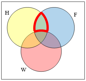
Image from Book Title by David Lippman, Pierce College. Licensed under CC BY-SA. View original
A survey asks 200 people "What beverage do you drink in the morning?", and offers these choices:
- Tea only
- Coffee only
- Both coffee and tea
Suppose 20 report tea only, 80 report coffee only, 40 report both.
Questions:
a) How many people drink tea in the morning?
b) How many people drink neither tea nor coffee?
Fifty students were surveyed and asked if they were taking a social science (SS), humanities (HM) or a natural science (NS) course the next quarter.
- 21 were taking a SS course
- 26 were taking a HM course
- 19 were taking a NS course
- 9 were taking SS and HM
- 7 were taking SS and NS
- 10 were taking HM and NS
- 3 were taking all three
- 7 were taking none
Question: How many students are taking only a SS course?
Problems adapted from David Lippman, Pierce College. Licensed under CC BY-SA.
PubMed/MeSH
PubMed: Building a Search
Learn a systematic approach to find relevant articles on a given topic in PubMed combined with Mesh
PubMed is a free search engine maintained by the U.S. National Library of Medicine (NLM) that gives you access to more than 39 million citations from biomedical and life-science literature
PubMed
├── Search
│ ├── Basic Search
│ └── Advanced Search
│ └── MeSH Search
│
├── Filters
│ ├── Year
│ ├── Article Type
│ └── Free Full Text
│
├── Databases
│ ├── MEDLINE
│ ├── PubMed Central
│ └── Bookshelf
│
└── Article Page
├── Citation
├── Abstract
├── MeSH Terms
└── Links to Full Text
What is Mesh DB?
Mesh terms are like tags attached to research papers. You can access Mesh database from this link https://www.ncbi.nlm.nih.gov/mesh/.
MeSH DB (Medical Subject Headings Database) is a controlled vocabulary system used to tag, organize, and standardize biomedical topics for precise searching in PubMed.

Be carefull for the Major topic or just Mesh Term or maybe sub-term asked in the question like AD diagnosis and not only AD.
See this sites for all tags and terms https://pubmed.ncbi.nlm.nih.gov/help/#using-search-field-tags
Protein Databases
Protein databases store information about protein structures, sequences, and functions. They come from experimental methods or computational predictions.
PDB
What is PDB? PDB (Protein Data Bank) is the main global database that stores 3D structures of proteins, DNA, RNA, and their complexes.
How experimental structure data is obtained? (3 methods)
- X-ray Crystallography(88%): uses crystals + X-ray diffraction to map atomic positions.
- NMR Spectroscopy(10%): uses magnetic fields to determine structures in solution.
- Cryo-Electron Microscopy (Cryo-EM)(1%)
What is a Ligand?: A ligand is any small molecule, ion, or cofactor that binds to the protein in the structure, often to perform a specific biological function. Example: iron in hemoglobin
What is Resolution (Å)? Resolution (in Ångström) measures the level of detail; smaller value = sharper, more accurate structure.
What is the PDB? (Again)
The Protein Data Bank is the central repository for 3D structures of biological macromolecules (proteins, DNA, RNA). If you want to know what a protein looks like in 3D, you go to PDB.
Current stats:
- ~227,000 experimental structures
- ~1,000,000+ computed structure models (AlphaFold)
The wwPDB Consortium
wwPDB (worldwide Protein Data Bank) was established in 2003. Three data centers maintain it:
| Center | Location | Website |
|---|---|---|
| RCSB PDB | USA | rcsb.org |
| PDBe | Europe (EMBL-EBI) | ebi.ac.uk/pdbe |
| PDBj | Japan | pdbj.org |
They all share the same data, but each has different tools and interfaces.
What wwPDB Does
- Structure deposition — researchers submit their structures through OneDep (deposit.wwpdb.org)
- Structure validation — quality checking before release
- Structure archive — maintaining the database
Related Archives
| Archive | What it stores |
|---|---|
| PDB | Atomic coordinates |
| EMDB | Electron microscopy density maps |
| BMRB | NMR data (chemical shifts, restraints) |
SIFTS
SIFTS (Structure Integration with Function, Taxonomy and Sequence) provides residue-level mapping between:
- PDB entries ↔ UniProt sequences
- Connections to: GO, InterPro, Pfam, CATH, SCOP, PubMed, Ensembl
This is how you can search PDB by Pfam domain or UniProt ID.
Part 1: Experimental Methods
Three main methods to determine protein structures:
| Method | % of PDB (2017) | Size limit | Resolution |
|---|---|---|---|
| X-ray crystallography | 88% | None | Can be <1 Å |
| NMR spectroscopy | 10% | <50-70 kDa | N/A |
| Cryo-EM | 1% (now ~10%) | >50 kDa | Rarely <2.2 Å |
Important: Cryo-EM has grown exponentially since 2017 due to the "Resolution Revolution."
X-ray Crystallography
The Process
Protein → Crystallize → X-ray beam → Diffraction pattern →
Electron density map → Atomic model
- Crystallization — grow protein crystals (ordered molecular packing)
- X-ray diffraction — shoot X-rays at the crystal
- Diffraction pattern — X-rays scatter, creating spots on detector
- Phase determination — the "phase problem" (you measure intensities but need phases)
- Electron density map — Fourier transform gives you electron density
- Model fitting — build atomic model into the density
Why X-rays?
Wavelength matters:
- Visible light: λ ≈ 10⁻⁵ cm — too big to resolve atoms
- X-rays: λ ≈ 10⁻⁸ cm — comparable to atomic distances (~1-2 Å)
Problem: No lens can focus X-rays. Computers must calculate the inverse Fourier transform.
Why Crystals?
A single molecule gives too weak a signal. Crystals contain millions of molecules in identical orientations, amplifying the diffraction signal.
The Phase Problem
When X-rays scatter, you measure:
- Amplitudes |F(hkl)| — from diffraction spot intensities ✓
- Phases α(hkl) — LOST in the measurement ✗
Phases must be determined indirectly (molecular replacement, heavy atom methods, etc.). This is why X-ray crystallography is hard.
Resolution
Definition: The smallest detail you can see in the structure.
What limits resolution: If molecules in the crystal aren't perfectly aligned (due to flexibility or disorder), fine details are lost.
| Resolution | Quality | What you can see |
|---|---|---|
| 0.5-1.5 Å | Exceptional | Individual atoms, hydrogens sometimes visible |
| 1.5-2.5 Å | High | Most features clear, good for detailed analysis |
| 2.5-3.5 Å | Medium | Overall fold clear, some ambiguity in sidechains |
| >3.5 Å | Low | Only general shape, significant uncertainty |
Lower number = better resolution. A 1.5 Å structure is better than a 3.0 Å structure.
Cryo-Electron Microscopy (Cryo-EM)
The Resolution Revolution
Nobel Prize in Chemistry 2017. Progress on β-Galactosidase:
| Year | Resolution |
|---|---|
| 2005 | 25 Å (blob) |
| 2011 | 11 Å |
| 2013 | 6 Å |
| 2014 | 3.8 Å |
| 2015 | 2.2 Å |
The Process
Protein → Flash-freeze in vitreous ice → Image thousands of particles →
Align and average → 3D reconstruction → Build model
- Sample preparation — purify protein, flash-freeze in thin ice layer
- Imaging — electron beam through frozen sample
- Data collection — thousands of images of individual particles
- Image processing — classify, align, and average particles
- 3D reconstruction — combine to get density map
- Model building — fit atomic model into density
Advantages
- No crystals needed — works on samples that won't crystallize
- Large complexes — good for ribosomes, viruses, membrane proteins
- Multiple conformations — can separate different states
Limitations
- Size limit: Generally requires proteins >50 kDa (small proteins are hard to image)
- Resolution: Very rarely reaches below ~2.2 Å
NMR Spectroscopy
How It Works
NMR doesn't give you a single structure. It gives you restraints (constraints):
- Dihedral angles — backbone and sidechain torsion angles
- Inter-proton distances — from NOE (Nuclear Overhauser Effect)
- Other restraints — hydrogen bonds, orientations
The Output
NMR produces a bundle of structures (ensemble), all compatible with the restraints.
Model 1
/
Restraints → Model 2 → All satisfy the experimental data
\
Model 3
A reference structure can be calculated by averaging.
What Does Variation Mean?
When NMR models differ from each other, it could mean:
- Real flexibility — the protein actually moves
- Uncertainty — not enough data to pin down the position
This is ambiguous and requires careful interpretation.
Advantages
- Dynamics — can observe protein folding, conformational changes
- Solution state — protein in solution, not crystal
Limitations
- Size limit: ≤50-70 kDa (larger proteins have overlapping signals)
Method Comparison Summary
| Feature | X-ray | Cryo-EM | NMR |
|---|---|---|---|
| Sample | Crystal required | Frozen in ice | Solution |
| Size limit | None | >50 kDa | <50-70 kDa |
| Resolution | Can be <1 Å | Rarely <2.2 Å | N/A |
| Dynamics | No | Limited | Yes |
| Multiple states | Difficult | Yes | Yes |
| Membrane proteins | Difficult | Good | Limited |
Part 2: AlphaFold and Computed Structure Models
Timeline
| Method | First structure | Nobel Prize |
|---|---|---|
| X-ray | 1958 | 1962 |
| NMR | 1988 | 2002 |
| Cryo-EM | 2014 | 2017 |
| AlphaFold | 2020 | 2024 |
What is AlphaFold?
A deep learning system that predicts protein structure from sequence.
Amino acid sequence → AlphaFold neural network → 3D structure prediction
How It Works
Input features:
-
MSA (Multiple Sequence Alignment) — find related sequences in:
- UniRef90 (using jackhmmer)
- Mgnify (metagenomic sequences)
- BFD (2.5 billion proteins)
-
Template structures — search PDB70 for similar known structures
Key concept: Co-evolution
If two positions in a protein always mutate together across evolution, they're probably in contact in 3D.
Example:
Position 3: R, R, R, K, K, K (all positive)
Position 9: D, D, D, E, E, E (all negative)
These positions probably form a salt bridge.
AlphaFold Performance
At CASP14 (2020), AlphaFold2 scored ~92 GDT (Global Distance Test).
- GDT > 90 ≈ experimental structure accuracy
- Previous best methods: 40-60 GDT
AlphaFold essentially solved the protein folding problem for single domains.
AlphaFold Database
- Created: July 2021
- Current size: ~214 million structures
- Coverage: 48 complete proteomes (including human)
- Access: UniProt, RCSB PDB, Ensembl
AlphaFold Confidence Metrics
These are critical for interpreting AlphaFold predictions.
pLDDT (predicted Local Distance Difference Test)
Stored in the B-factor column of AlphaFold PDB files.
| pLDDT | Confidence | Interpretation |
|---|---|---|
| >90 | Very high | Side chains reliable, can analyze active sites |
| 70-90 | Confident | Backbone reliable |
| 50-70 | Low | Uncertain |
| <50 | Very low | Likely disordered, NOT a structure prediction |
What pLDDT measures: Confidence in local structure (not global fold).
Uses:
- Identify structured domains vs disordered regions
- Decide which parts to trust
PAE (Predicted Aligned Error)
A 2D matrix showing confidence in relative positions between residues.
Residue j →
┌─────────────────┐
R │ ■■■ ░░░ │ ■ = low error (confident)
e │ ■■■ ░░░ │ ░ = high error (uncertain)
s │ │
i │ ■■■■■ │
d │ ■■■■■ │
u │ │
e │ ░░░░░░ │
i ↓ │ ░░░░░░ │
└─────────────────┘
Dark blocks on diagonal: Confident domains Off-diagonal dark blocks: Confident domain-domain interactions Light regions: Uncertain relative positions (domains may be connected but orientation unknown)
Use PAE for: Determining if domain arrangements are reliable.
Part 3: PDB File Formats
Legacy PDB Format
ATOM 1 N LYS A 1 -21.816 -8.515 19.632 1.00 41.97
ATOM 2 CA LYS A 1 -20.532 -9.114 20.100 1.00 41.18
| Column | Meaning |
|---|---|
| ATOM | Record type |
| 1, 2 | Atom serial number |
| N, CA | Atom name |
| LYS | Residue name |
| A | Chain ID |
| 1 | Residue number |
| -21.816, -8.515, 19.632 | X, Y, Z coordinates (Å) |
| 1.00 | Occupancy |
| 41.97 | B-factor |
mmCIF Format
Current standard. More flexible than legacy PDB format:
- Can handle >99,999 atoms
- Machine-readable
- Extensible
The B-factor Column
The B-factor means different things depending on the method:
| Method | B-factor contains | Meaning |
|---|---|---|
| X-ray | Temperature factor | Atomic mobility/disorder |
| NMR | RMSF | Fluctuation across models |
| AlphaFold | pLDDT | Prediction confidence |
For X-ray: $$B = 8\pi^2 U^2$$
Where U² is mean square displacement.
| B-factor | Displacement | Interpretation |
|---|---|---|
| 15 Ų | ~0.44 Š| Rigid |
| 60 Ų | ~0.87 Š| Flexible |
Part 4: Data Validation
Why Validation Matters
Not all PDB structures are equal quality. You need to check:
- Resolution (for X-ray/Cryo-EM)
- R-factors (for X-ray)
- Geometry (for all)
Resolution
Most important quality indicator for X-ray and Cryo-EM.
Lower = better. A 1.5 Å structure shows more detail than a 3.0 Å structure.
R-factor (X-ray only)
Measures how well the model fits the experimental data.
$$R = \frac{\sum |F_{obs} - F_{calc}|}{\sum |F_{obs}|}$$
| R-factor | Interpretation |
|---|---|
| <0.20 | Good fit |
| 0.20-0.25 | Acceptable |
| >0.30 | Significant errors likely |
Types of R-factors:
- R-work: Calculated on data used for refinement
- R-free: Calculated on test set NOT used for refinement (more honest)
R-free is more reliable. If R-work is much lower than R-free, the model may be overfitted.
Geometry Validation
| Metric | What it checks |
|---|---|
| Clashscore | Steric clashes between atoms |
| Ramachandran outliers | Unusual backbone angles (φ/ψ) |
| Sidechain outliers | Unusual rotamer conformations |
| RSRZ outliers | Residues that don't fit electron density |
RSRZ: Real Space R-value Z-score
- Measures fit between residue and electron density
- RSRZ > 2 = outlier
wwPDB Validation Report
Every PDB entry has a validation report with:
- Overall quality metrics
- Chain-by-chain analysis
- Residue-level indicators
- Color coding (green = good, red = bad)
Always check the validation report before trusting a structure!
Part 5: Advanced Search in RCSB PDB
Query Builder Categories
-
Attribute Search
- Structure attributes (method, resolution, date)
- Chemical attributes (ligands)
- Full text
-
Sequence-based Search
- Sequence similarity (BLAST)
- Sequence motif
-
Structure-based Search
- 3D shape similarity
- Structure motif
-
Chemical Search
- Ligand similarity
Key Search Fields
| Field | Use for |
|---|---|
| Experimental Method | "X-RAY DIFFRACTION", "ELECTRON MICROSCOPY", "SOLUTION NMR" |
| Data Collection Resolution | X-ray resolution |
| Reconstruction Resolution | Cryo-EM resolution |
| Source Organism | Species |
| UniProt Accession | Link to UniProt |
| Pfam Identifier | Domain family |
| CATH Identifier | Structure classification |
| Reference Sequence Coverage | How much of UniProt sequence is in structure |
Boolean Logic
AND — both conditions must be true
OR — either condition can be true
Important: When combining different resolution types, use OR correctly.
Practice Exercises
Exercise 1: Pfam Domain Search
Find X-ray structures at resolution ≤2.5 Å, from human and mouse, containing Pfam domain PF00004.
Query:
Experimental Method = "X-RAY DIFFRACTION"
AND Identifier = "PF00004" AND Annotation Type = "Pfam"
AND (Source Organism = "Homo sapiens" OR Source Organism = "Mus musculus")
AND Data Collection Resolution <= 2.5
Answer: 11-50 (15 entries)
Exercise 2: UniProt ID List with Filters
Find X-ray structures for a list of UniProt IDs, with resolution ≤2.2 Å and sequence coverage ≥0.90.
Query:
Accession Code(s) IS ANY OF [list of UniProt IDs]
AND Database Name = "UniProt"
AND Experimental Method = "X-RAY DIFFRACTION"
AND Data Collection Resolution <= 2.2
AND Reference Sequence Coverage >= 0.9
Answer: 501-1000 (811 entries)
Note: "Reference Sequence Coverage" tells you what fraction of the UniProt sequence is present in the PDB structure. Coverage of 0.90 means at least 90% of the protein is in the structure.
Exercise 3: Combining X-ray and Cryo-EM
Find all X-ray structures with resolution ≤2.2 Å AND all Cryo-EM structures with reconstruction resolution ≤2.2 Å.
The tricky part: X-ray uses "Data Collection Resolution" but Cryo-EM uses "Reconstruction Resolution". You need to combine them correctly.
Query:
(Experimental Method = "X-RAY DIFFRACTION" OR Experimental Method = "ELECTRON MICROSCOPY")
AND (Data Collection Resolution <= 2.2 OR Reconstruction Resolution <= 2.2)
Answer: 100001-1000000 (128,107 entries: 127,405 X-ray + 702 EM)
Why this works: Each entry will match either:
- X-ray AND Data Collection Resolution ≤2.2, OR
- EM AND Reconstruction Resolution ≤2.2
Exercise 4: Cryo-EM Quality Filter
Among Cryo-EM structures with resolution ≤2.2 Å, how many have Ramachandran outliers <1%?
Query:
Experimental Method = "ELECTRON MICROSCOPY"
AND Reconstruction Resolution <= 2.2
AND Molprobity Percentage Ramachandran Outliers <= 1
Answer: 101-1000 (687 out of 702 total)
This tells you that most high-resolution Cryo-EM structures have good geometry.
Query Building Tips
1. Use the Right Resolution Field
| Method | Resolution Field |
|---|---|
| X-ray | Data Collection Resolution |
| Cryo-EM | Reconstruction Resolution |
| NMR | N/A (no resolution) |
2. Experimental Method Exact Names
Use exactly:
"X-RAY DIFFRACTION"(not "X-ray" or "crystallography")"ELECTRON MICROSCOPY"(not "Cryo-EM" or "EM")"SOLUTION NMR"(not just "NMR")
3. Organism Names
Use full taxonomic name:
"Homo sapiens"(not "human")"Mus musculus"(not "mouse")"Rattus norvegicus"(not "rat")
4. UniProt Queries
When searching by UniProt ID, specify:
Accession Code = [ID] AND Database Name = "UniProt"
5. Combining OR Conditions
Always put OR conditions in parentheses:
(Organism = "Homo sapiens" OR Organism = "Mus musculus")
Otherwise precedence may give unexpected results.
What to Check When Using a PDB Structure
- Experimental method — X-ray? NMR? Cryo-EM?
- Resolution — <2.5 Å is generally good for most purposes
- R-factors — R-free should be reasonable for the resolution
- Validation report — check for outliers in your region of interest
- Sequence coverage — does the structure include the region you care about?
- Ligands/cofactors — are they present? Are they what you expect?
Comparing Experimental vs AlphaFold Structures
When AlphaFold structures are available:
| Check | Experimental | AlphaFold |
|---|---|---|
| Overall reliability | Resolution, R-factor | pLDDT, PAE |
| Local confidence | B-factor (flexibility) | pLDDT (prediction confidence) |
| Disordered regions | Often missing | Low pLDDT (<50) |
| Ligand binding sites | Can have ligands | No ligands |
| Protein-protein interfaces | Shown in complex structures | Not reliable unless AlphaFold-Multimer |
Key insight: Low-confidence AlphaFold regions often correspond to regions missing in experimental structures — both are telling you the same thing (disorder/flexibility).
Quick Reference
PDB Quality Indicators
| Indicator | Good value | Bad value |
|---|---|---|
| Resolution | <2.5 Å | >3.5 Å |
| R-free | <0.25 | >0.30 |
| Ramachandran outliers | <1% | >5% |
| Clashscore | <5 | >20 |
AlphaFold Confidence
| pLDDT | Meaning |
|---|---|
| >90 | Very confident, analyze details |
| 70-90 | Confident backbone |
| 50-70 | Low confidence |
| <50 | Likely disordered |
Search Field Cheatsheet
| What you want | Field to use |
|---|---|
| X-ray resolution | Data Collection Resolution |
| Cryo-EM resolution | Reconstruction Resolution |
| Species | Source Organism Taxonomy Name |
| UniProt link | Accession Code + Database Name = "UniProt" |
| Pfam domain | Identifier + Annotation Type = "Pfam" |
| CATH superfamily | Lineage Identifier (CATH) |
| Coverage | Reference Sequence Coverage |
| Geometry quality | Molprobity Percentage Ramachandran Outliers |
For the Oral Exam
Be prepared to explain:
-
Why crystallography needs crystals — signal amplification from ordered molecular packing
-
The phase problem — you measure amplitudes but lose phases; must determine indirectly
-
What resolution means — ability to distinguish fine details; limited by crystal order
-
Why Cryo-EM grew so fast — no crystals needed, good for large complexes, computational advances
-
NMR gives ensembles, not single structures — restraints satisfied by multiple conformations
-
What pLDDT means — local prediction confidence, stored in B-factor column
-
Difference between pLDDT and PAE — pLDDT is local confidence, PAE is relative domain positioning
-
How to assess structure quality — resolution, R-factors, validation metrics
-
B-factor means different things — mobility (X-ray), fluctuation (NMR), confidence (AlphaFold)
-
How to construct complex PDB queries — combining method, resolution, organism, domain annotations
UCSF-Chimera
Short Playlist:
So you need to visualize protein structures, analyze binding sites, or understand why a mutation causes disease? Welcome to Chimera — your molecular visualization workhorse.
What is Chimera?
UCSF Chimera — a free molecular visualization program from UC San Francisco. It lets you:
- Visualize 3D protein/DNA/RNA structures
- Analyze protein-ligand interactions
- Measure distances and angles
- Compare structures (superposition)
- Color by various properties (charge, hydrophobicity, conservation, flexibility)
- Generate publication-quality images
Getting Started
Opening a Structure
From PDB (online):
File → Fetch by ID → Enter PDB code (e.g., 1a6m) → Fetch
From file:
File → Open → Select your .pdb file
Representation Styles
The Main Styles
| Style | What it shows | Use for |
|---|---|---|
| Ribbon/Cartoon | Secondary structure (helices, sheets) | Overall fold |
| Sticks | All bonds as sticks | Detailed view of residues |
| Ball and Stick | Atoms as balls, bonds as sticks | Ligands, active sites |
| Sphere/Spacefill | Atoms as van der Waals spheres | Space-filling, surfaces |
| Wire | Thin lines for bonds | Large structures |
How to Change Representation
Actions → Atoms/Bonds → [stick/ball & stick/sphere/wire]
Actions → Ribbon → [show/hide]
Ribbon for protein backbone + Sticks for ligand/active site residues = best of both worlds
Selection: The Most Important Skill
Everything in Chimera starts with selection. Select what you want, then do something to it.
Selection Methods
| Method | How | Example |
|---|---|---|
| Click | Ctrl + Click on atom | Select one atom |
| Menu | Select → ... | Various options |
| Chain | Select → Chain → A | Select chain A |
| Residue type | Select → Residue → HIS | All histidines |
| Command line | select :153 | Residue 153 |
Useful Selection Menu Options
Select → Chain → [A, B, C...] # Select by chain
Select → Residue → [ALA, HIS, IHP...] # Select by residue type
Select → Structure → Protein # All protein
Select → Structure → Ligand # All ligands
Select → Chemistry → Side chain # Just sidechains
Select → Clear Selection # Deselect everything
Select → Invert (all models) # Select everything NOT selected
Zone Selection (Within Distance)
Select everything within X Å of current selection:
Select → Zone...
→ Set distance (e.g., 6 Å)
→ OK
This is super useful for finding binding site residues!
Coloring
Color by Element (Default)
Actions → Color → by element
| Element | Color |
|---|---|
| Carbon | Gray |
| Oxygen | Red |
| Nitrogen | Blue |
| Sulfur | Yellow |
| Hydrogen | White |
| Iron | Orange-brown |
| Phosphorus | Orange |
Color by Hydrophobicity
Tools → Depiction → Render by Attribute
→ Attribute: kdHydrophobicity
→ OK
| Color | Meaning |
|---|---|
| Blue/Cyan | Hydrophilic (polar) |
| White | Intermediate |
| Orange/Red | Hydrophobic (nonpolar) |
Why use this? To see the hydrophobic core of proteins — nonpolar residues hide inside, polar residues face the water.
Color by Electrostatic Potential (Coulombic)
This is the red-white-blue coloring from your exercise!
Step 1: Generate surface first
Actions → Surface → Show
Step 2: Color by charge
Tools → Surface/Binding Analysis → Coulombic Surface Coloring → OK
| Color | Charge | Attracts... |
|---|---|---|
| Blue | Positive (+) | Negative molecules |
| Red | Negative (−) | Positive molecules |
| White | Neutral | Hydrophobic stuff |
The OK button is disabled if no surface exists. Always do Actions → Surface → Show first!
What to look for:
- Binding pockets often have complementary charge to ligand
- DNA-binding proteins have positive (blue) surfaces to attract negative DNA
- Negatively charged ligands (like phosphates) bind in positive (blue) pockets
Color by B-factor (Flexibility)
B-factor = temperature factor = how much an atom "wiggles" in the crystal.
Tools → Depiction → Render by Attribute
→ Attribute: bfactor
→ OK
| Color | B-factor | Meaning |
|---|---|---|
| Blue | Low | Rigid, well-ordered |
| Red | High | Flexible, mobile |
What to expect:
- Protein core: Blue (rigid)
- Loops and termini: Red (floppy)
- Active sites: Often intermediate
Color by Conservation
When you have multiple aligned structures:
Tools → Sequence → Multialign Viewer
→ (structures get aligned)
Structure → Render by Conservation
| Color | Conservation |
|---|---|
| Blue/Purple | Highly conserved |
| Red | Variable |
Conserved residues = functionally important (active sites, structural core)
Molecular Surfaces
Show/Hide Surface
Actions → Surface → Show
Actions → Surface → Hide
Transparency
Actions → Surface → Transparency → [0-100%]
Use ~50-70% transparency to see ligands through the surface.
Cross-Section (Clipping)
To see inside the protein:
Tools → Depiction → Per-Model Clipping
→ Enable clipping
→ Adjust plane position
Or use the Side View panel:
Tools → Viewing Controls → Side View
Measuring Distances
Method 1: Distance Tool
Tools → Structure Analysis → Distances
Then Ctrl+Shift+Click on first atom, Ctrl+Shift+Click on second atom.
Distance appears as a yellow dashed line with measurement.
Method 2: Command Line
distance :169@OG :301@O34
What Distances Mean
| Distance | Interaction Type |
|---|---|
| ~1.0–1.5 Å | Covalent bond |
| ~1.8–2.1 Å | Coordination bond (metal) |
| ~2.5–3.5 Å | Hydrogen bond |
| ~2.8–4.0 Å | Salt bridge |
| > 4 Å | No direct interaction |
Hydrogen Bonds
What is a Hydrogen Bond?
Donor—H · · · · Acceptor
↑
H-bond (~2.5-3.5 Å)
- Donor: Has hydrogen to give (—OH, —NH)
- Acceptor: Has lone pair to receive (O=, N)
Find H-Bonds Automatically
Tools → Structure Analysis → FindHBond
Options:
- ✓ Include intra-molecule (within protein)
- ✓ Include inter-molecule (protein-ligand)
H-bonds appear as blue/green lines.
Common H-Bond Donors in Proteins
| Amino Acid | Donor Atom | Group |
|---|---|---|
| Serine | OG | —OH |
| Threonine | OG1 | —OH |
| Tyrosine | OH | —OH |
| Histidine | NE2, ND1 | Ring —NH |
| Lysine | NZ | —NH₃⁺ |
| Arginine | NH1, NH2, NE | Guanidinium |
| Backbone | N | Amide —NH |
Common H-Bond Acceptors
| Group | Atoms |
|---|---|
| Phosphate | O atoms |
| Carboxylate | OD1, OD2 (Asp), OE1, OE2 (Glu) |
| Carbonyl | O (backbone) |
| Hydroxyl | O (can be both donor AND acceptor) |
Salt Bridges (Ionic Interactions)
A salt bridge = electrostatic attraction between opposite charges.
| Positive (basic) | Negative (acidic) |
|---|---|
| Lysine (NZ) | Aspartate (OD1, OD2) |
| Arginine (NH1, NH2) | Glutamate (OE1, OE2) |
| Histidine (when protonated) | C-terminus |
| N-terminus | Phosphate groups |
Typical distance: ~2.8–4.0 Å between charged atoms
Coordination Bonds (Metals)
Metals like Fe, Zn, Mg are coordinated by specific atoms:
| Metal | Common Ligands | Distance |
|---|---|---|
| Fe (heme) | His NE2, O₂ | ~2.0–2.2 Å |
| Zn | Cys S, His N | ~2.0–2.3 Å |
| Mg | Asp/Glu O, water | ~2.0–2.2 Å |
Example: In myoglobin (1a6m), the proximal histidine coordinates Fe at ~2.1 Å.
Ramachandran Plot
Shows allowed backbone angles (φ/ψ) for amino acids.
Tools → Structure Analysis → Ramachandran Plot
Regions of the Plot
| Region | Location | Structure |
|---|---|---|
| Lower left | φ ≈ -60°, ψ ≈ -45° | α-helix |
| Upper left | φ ≈ -120°, ψ ≈ +130° | β-sheet |
| Upper right | Positive φ | Left-handed helix (rare) |
Why Glycine is Special
Glycine has no sidechain → no steric clashes → can be in "forbidden" regions (positive φ).
Select → Residue → GLY
Glycines often appear in the right half of the Ramachandran plot where other residues can't go.
Structural Superposition
Compare two similar structures by overlaying them.
Method 1: MatchMaker (Sequence-based)
Tools → Structure Comparison → MatchMaker
→ Reference: structure 1
→ Match: structure 2
→ OK
Output tells you:
- RMSD (Root Mean Square Deviation): How well they align
- < 1 Å = very similar
- 1–2 Å = similar fold
-
3 Å = significant differences
- Sequence identity %: How similar the sequences are
Method 2: Match (Command)
match #1 #0
Restricting Alignment to a Region
To align just the active site (e.g., within 4 Å of ligand):
sel #1:hem #0:hem zr < 4
match sel
Working with Chains
Delete Unwanted Chains
Select → Chain → B
Actions → Atoms/Bonds → Delete
Select Specific Chain
Select → Chain → A
Or command:
select #0:.A
AlphaFold Structures and pLDDT
What is pLDDT?
AlphaFold stores its confidence score (pLDDT) in the B-factor column.
| pLDDT | Confidence | Typical regions |
|---|---|---|
| > 90 | Very high | Structured core |
| 70–90 | Confident | Most of protein |
| 50–70 | Low | Loops, uncertain |
| < 50 | Very low | Disordered regions |
Color by pLDDT
Since pLDDT is in B-factor column, use:
Tools → Depiction → Render by Attribute → bfactor
Or select low-confidence regions:
select @@bfactor<70
Low pLDDT regions in AlphaFold often correspond to regions that are ALSO missing in experimental structures — they're genuinely disordered/flexible, not just bad predictions.
The Hydrophobic Core
Soluble proteins organize with:
- Hydrophobic residues (Leu, Ile, Val, Phe, Met) → inside (core)
- Polar/charged residues (Lys, Glu, Ser, Asp) → outside (surface)
Visualizing the Core
- Color by hydrophobicity
- Use cross-section/clipping to see inside
- Orange/tan inside, blue/cyan outside = correct fold
Protein-Ligand Interaction Analysis
General Workflow
-
Isolate the binding site:
Select → Residue → [ligand name] Select → Zone → 5-6 Å -
Delete or hide everything else:
Select → Invert Actions → Atoms/Bonds → Delete (or Hide) -
Show interactions:
Tools → Structure Analysis → FindHBond -
Measure specific distances:
Tools → Structure Analysis → Distances -
Look at electrostatics:
Actions → Surface → Show Tools → Surface/Binding Analysis → Coulombic Surface Coloring
What to Report
For protein-ligand interactions, describe:
| Interaction Type | How to Identify |
|---|---|
| Hydrogen bonds | Distance 2.5–3.5 Å, involves N-H or O-H |
| Salt bridges | Opposite charges, distance ~2.8–4 Å |
| Hydrophobic | Nonpolar residues surrounding nonpolar parts of ligand |
| Coordination | Metal ion with specific geometry |
| Electrostatic complementarity | Blue pocket for negative ligand (or vice versa) |
Example: Analyzing a Binding Site (3eeb)
This is the exercise you did!
The Setup
1. Fetch 3eeb
2. Delete chain B (Select → Chain → B, then Delete)
3. Show surface, color by electrostatics
Result: Blue (positive) binding pocket for the negative IHP (6 phosphates).
The Details
1. Hide surface
2. Select IHP, then Zone 6 Å
3. Invert selection, Delete
4. Show sidechains, keep ribbon
5. Measure distances
Result:
- Ser 169 OG ↔ IHP O34: ~2.8 Å = hydrogen bond (Ser donates H)
- His 55 NE2 ↔ IHP O22: ~2.9 Å = hydrogen bond (His donates H)
The Interpretation
"IHP binding is driven by electrostatic attraction (positive pocket, negative ligand) and stabilized by specific hydrogen bonds from Ser 169 and His 55 to phosphate oxygens."
Cancer Mutations in p53 (1tup)
Example from your lectures showing how to analyze mutation hotspots:
The Hotspot Residues
| Residue | Type | Role |
|---|---|---|
| R248 | Contact | Directly touches DNA |
| R273 | Contact | Directly touches DNA |
| R175 | Structural | Stabilizes DNA-binding loop |
| H179 | Structural | Stabilizes DNA-binding loop |
Analysis Approach
1. Open 1tup, keep chain B
2. Show R175, R248, R273, H179 in spacefill
3. Color surface by electrostatics
Result:
- R248 and R273 are right at the DNA interface (positive surface touching negative DNA)
- R175 and H179 are buried, maintaining the fold
- Mutations here → lose DNA binding → lose tumor suppression → cancer
Common Chimera Workflows
Quick Look at a Structure
1. File → Fetch by ID
2. Actions → Ribbon → Show
3. Presets → Interactive 1 (ribbons)
4. Rotate, zoom, explore
Analyze Active Site
1. Select ligand
2. Select → Zone → 5 Å
3. Actions → Atoms/Bonds → Show (for selection)
4. Tools → Structure Analysis → FindHBond
Compare Two Structures
1. Open both structures
2. Tools → Structure Comparison → MatchMaker
3. Check RMSD and sequence identity
Make a Figure
1. Set up your view
2. Presets → Publication 1
3. File → Save Image
Command Line Quick Reference
The command line is at the bottom of the Chimera window. Faster than menus once you know commands.
| Command | What it does |
|---|---|
open 1a6m | Fetch and open PDB |
select :153 | Select residue 153 |
select :HIS | Select all histidines |
select #0:.A | Select chain A of model 0 |
select :hem zr<5 | Select within 5 Å of heme |
display sel | Show selected atoms |
~display ~sel | Hide unselected atoms |
color red sel | Color selection red |
represent sphere | Spacefill for selection |
distance :169@OG :301@O34 | Measure distance |
match #1 #0 | Superpose model 1 onto 0 |
surface | Show surface |
~surface | Hide surface |
del sel | Delete selection |
Keyboard Shortcuts
| Key | Action |
|---|---|
| Ctrl + Click | Select atom |
| Ctrl + Shift + Click | Add to selection / measure distance |
| Scroll wheel | Zoom |
| Right-drag | Translate |
| Left-drag | Rotate |
| Middle-drag | Zoom (alternative) |
Troubleshooting Common Issues
"Nothing selected"
You tried to do something but nothing happened:
- Check: Is anything actually selected? (Green highlighting)
- Fix: Select → [what you want] first
Surface coloring disabled
- Check: Does a surface exist?
- Fix:
Actions → Surface → Showfirst
Can't see ligand
- Check: Is it hidden?
- Fix:
Select → Residue → [ligand], thenActions → Atoms/Bonds → Show
Structure looks weird after operations
- Fix:
Presets → Interactive 1to reset to default view
Atoms showing when you want ribbon only
Actions → Atoms/Bonds → Hide
Actions → Ribbon → Show
External Resources for Structure Analysis
| Resource | URL | Use for |
|---|---|---|
| RCSB PDB | rcsb.org | US PDB, structure info |
| PDBe | ebi.ac.uk/pdbe | European PDB, ligand interactions |
| PLIP | plip-tool.biotec.tu-dresden.de | Automated interaction analysis |
| AlphaFold DB | alphafold.ebi.ac.uk | Predicted structures |
| COSMIC | cancer.sanger.ac.uk/cosmic | Cancer mutations |
TL;DR
| Task | How |
|---|---|
| Open structure | File → Fetch by ID |
| Select | Select → [Chain/Residue/Zone] |
| Delete | Select, then Actions → Atoms/Bonds → Delete |
| Show surface | Actions → Surface → Show |
| Color by charge | Surface first, then Tools → Surface/Binding Analysis → Coulombic |
| Color by flexibility | Tools → Depiction → Render by Attribute → bfactor |
| Measure distance | Tools → Structure Analysis → Distances, then Ctrl+Shift+Click |
| Find H-bonds | Tools → Structure Analysis → FindHBond |
| Compare structures | Tools → Structure Comparison → MatchMaker |
Key distances:
- ~2.0 Å = coordination bond
- ~2.5–3.5 Å = hydrogen bond
- ~2.8–4.0 Å = salt bridge
Electrostatic colors:
- Blue = positive
- Red = negative
- White = neutral
Now go visualize some proteins! 🧬
UniProt
Introduction
So you need protein sequences, functions, domains, or disease associations? Welcome to UniProt — the world's most comprehensive protein database, and your one-stop shop for everything protein-related.
Universal Protein Resource — a collaboration between three major institutions since 2002:
| Institution | Location | Contribution |
|---|---|---|
| SIB | Swiss Institute of Bioinformatics, Lausanne | UniProtKB/Swiss-Prot |
| EBI | European Bioinformatics Institute, UK | UniProtKB/TrEMBL, UniParc |
| PIR | Protein Information Resource, Georgetown | UniRef |
What it gives you:
- Protein sequences and functions
- Domains, families, PTMs
- Disease associations and variants
- Subcellular localization
- Cross-references to 180+ external databases
- Proteomes for complete organisms
- BLAST, Align, ID mapping tools
The UniProt Structure
UniProt isn't just one database — it's a collection:
UniProt
│
┌───────────────┼───────────────┐
│ │ │
UniProtKB UniRef UniParc
(Knowledge) (Clusters) (Archive)
│
┌───┴───┐
│ │
Swiss-Prot TrEMBL
(Reviewed) (Unreviewed)
| Database | What it is | Size (approx.) |
|---|---|---|
| Swiss-Prot | Manually curated, reviewed | ~570,000 entries |
| TrEMBL | Automatically annotated | ~250,000,000 entries |
| UniRef | Clustered sequences (100%, 90%, 50% identity) | Reduced redundancy |
| UniParc | Complete archive of all sequences | Non-redundant archive |
| Proteomes | Complete protein sets per organism | ~160,000 proteomes |
Swiss-Prot vs TrEMBL: Know the Difference
This is the most important distinction in UniProt:
| Aspect | Swiss-Prot (Reviewed) | TrEMBL (Unreviewed) |
|---|---|---|
| Curation | Manually reviewed by experts | Computationally analyzed |
| Data source | Scientific publications | Sequence repositories |
| Isoforms | Grouped together per gene | Individual entries |
| Quality | High confidence | Variable |
| Size | ~570K entries | ~250M entries |
| Icon | ⭐ Gold star | 📄 Document |
When you need reliable annotations, always add reviewed:true to your query. TrEMBL entries can be useful for breadth, but Swiss-Prot entries are gold standard.
UniProt Identifiers
Accession Numbers
The primary identifier — stable and persistent:
P05067 (6 characters: 1 letter + 5 alphanumeric)
A0A024RBG1 (10 characters: newer format)
Entry Names
Human-readable format: GENE_SPECIES
APP_HUMAN → Amyloid precursor protein, Human
INS_HUMAN → Insulin, Human
SPIKE_SARS2 → Spike protein, SARS-CoV-2
Accession (P05067) = stable, use for databases and scripts
Entry name (APP_HUMAN) = readable, can change if gene name updates
Protein Existence Levels
UniProt classifies how confident we are that a protein actually exists:
| Level | Evidence | Description |
|---|---|---|
| 1 | Protein level | Experimental evidence (MS, X-ray, etc.) |
| 2 | Transcript level | mRNA evidence, no protein detected |
| 3 | Homology | Inferred from similar sequences |
| 4 | Predicted | Gene prediction, no other evidence |
| 5 | Uncertain | Dubious, may not exist |
Query syntax: existence:1 (for protein-level evidence)
Annotation Score
A 1-5 score indicating annotation completeness (not accuracy!):
| Score | Meaning |
|---|---|
| 5/5 | Well-characterized, extensively annotated |
| 4/5 | Good annotation coverage |
| 3/5 | Moderate annotation |
| 2/5 | Basic annotation |
| 1/5 | Minimal annotation |
A score of 5/5 means the entry has lots of annotations — it doesn't guarantee they're all correct. A score of 1/5 might just mean the protein hasn't been studied much yet.
UniProt Search Syntax
UniProt uses a field-based query syntax. The general format:
field:value
Basic Query Structure
term1 AND term2 AND (term3 OR term4)
Boolean operators: AND, OR, NOT (can be uppercase or lowercase)
Key Search Fields
Organism and Taxonomy
| Field | Example | Description |
|---|---|---|
organism_name | organism_name:human | Search by name |
organism_id | organism_id:9606 | Search by NCBI taxonomy ID |
taxonomy_id | taxonomy_id:9606 | Same as organism_id |
Common taxonomy IDs:
- Human:
9606 - Mouse:
10090 - Rat:
10116 - Zebrafish:
7955 - E. coli K12:
83333 - Yeast:
559292
Review Status and Existence
| Field | Example | Description |
|---|---|---|
reviewed | reviewed:true | Swiss-Prot only |
reviewed | reviewed:false | TrEMBL only |
existence | existence:1 | Protein-level evidence |
Enzyme Classification (EC Numbers)
| Field | Example | Description |
|---|---|---|
ec | ec:3.4.21.1 | Exact EC number |
ec | ec:3.4.21.* | Wildcard for all serine endopeptidases |
ec | ec:3.4.* | All peptidases |
Use * as wildcard: ec:3.4.21.* matches all serine endopeptidases (3.4.21.1, 3.4.21.2, etc.)
Proteomes
| Field | Example | Description |
|---|---|---|
proteome | proteome:UP000005640 | Human reference proteome |
proteome | proteome:UP000000589 | Mouse reference proteome |
Finding proteome IDs: Go to UniProt → Proteomes → Search your organism
Cross-References (External Databases)
| Field | Example | Description |
|---|---|---|
database | database:pdb | Has PDB structure |
database | database:smr | Has Swiss-Model structure |
database | database:ensembl | Has Ensembl cross-ref |
xref | xref:pdb-1abc | Specific PDB ID |
Function and Annotation
| Field | Example | Description |
|---|---|---|
cc_function | cc_function:"ion transport" | Function comment |
cc_scl_term | cc_scl_term:SL-0039 | Subcellular location term |
keyword | keyword:kinase | UniProt keyword |
family | family:kinase | Protein family |
Gene Ontology
| Field | Example | Description |
|---|---|---|
go | go:0007155 | Any GO term (by ID) |
go | go:"cell adhesion" | Any GO term (by name) |
goa | goa:0007155 | GO annotation (same as go) |
Sequence Properties
| Field | Example | Description |
|---|---|---|
length | length:[100 TO 500] | Sequence length range |
mass | mass:[10000 TO 50000] | Molecular weight range |
cc_mass_spectrometry | cc_mass_spectrometry:* | Has MS data |
Building Complex Queries
Pattern 1: Reviewed + Organism + Function
reviewed:true AND organism_id:9606 AND cc_function:"kinase"
Pattern 2: Multiple EC Numbers
(ec:3.4.21.*) OR (ec:3.4.22.*)
Pattern 3: Multiple Organisms
(organism_id:10116) OR (organism_id:7955)
Pattern 4: Proteome + Database Cross-Reference
proteome:UP000005640 AND (database:pdb OR database:smr) AND reviewed:true
Pattern 5: Complex Boolean Logic
For "exactly two of three conditions" (A, B, C):
((A AND B) OR (B AND C) OR (A AND C)) NOT (A AND B AND C)
Practice Exercises
Exercise 1: Protein Existence Statistics
Q: (1) What percentage of TrEMBL entries have evidence at "protein level"? (2) What percentage of Swiss-Prot entries have evidence at "protein level"?
Click for answer
Answers:
- TrEMBL: ~0.17% (343,595 / 199,006,239)
- Swiss-Prot: ~20.7% (118,866 / 573,661)
Queries:
(1) (existence:1) AND (reviewed:false)
(2) (existence:1) AND (reviewed:true)
Takeaway: Swiss-Prot has ~100x higher percentage of experimentally verified proteins — that's why manual curation matters!
Exercise 2: EC Numbers + Multiple Organisms
Q: Retrieve all reviewed proteins annotated as either:
- Cysteine endopeptidases (EC 3.4.22.*)
- Serine endopeptidases (EC 3.4.21.*)
From: Rattus norvegicus [10116] and Danio rerio [7955]
How many?
Click for answer
Answer: 132 entries (121 rat, 11 zebrafish)
Query:
((ec:3.4.21.*) OR (ec:3.4.22.*)) AND ((organism_id:10116) OR (organism_id:7955)) AND (reviewed:true)
How to build it:
| Requirement | Query Component |
|---|---|
| Serine OR Cysteine peptidases | (ec:3.4.21.*) OR (ec:3.4.22.*) |
| Rat OR Zebrafish | (organism_id:10116) OR (organism_id:7955) |
| Reviewed only | reviewed:true |
⚠️ Watch the parentheses! Without proper grouping, you'll get wrong results.
Exercise 3: Proteome + Structure Cross-References
Q: Retrieve all reviewed entries from the Human Reference Proteome that have either:
- A PDB structure, OR
- A Swiss-Model Repository structure
How many?
Click for answer
Answer: 17,695 entries
Query:
proteome:UP000005640 AND ((database:pdb) OR (database:smr)) AND (reviewed:true)
Components:
| Requirement | Query |
|---|---|
| Human Reference Proteome | proteome:UP000005640 |
| PDB OR SMR structure | (database:pdb) OR (database:smr) |
| Reviewed | reviewed:true |
Exercise 4: Complex Boolean — "Exactly Two of Three"
Q: Find all reviewed entries with exactly two of these three properties:
- Function: "ion transport" (CC field)
- Subcellular location: "cell membrane" (SL-0039)
- GO term: "cell adhesion" (GO:0007155)
Click for answer
Answer: 2,022 entries
Query:
(cc_function:"ion transport" AND cc_scl_term:SL-0039) OR (cc_scl_term:SL-0039 AND go:0007155) OR (cc_function:"ion transport" AND go:0007155) NOT (cc_function:"ion transport" AND cc_scl_term:SL-0039 AND go:0007155) AND (reviewed:true)
Logic breakdown:
"Exactly two of three" = (A AND B) OR (B AND C) OR (A AND C), but NOT (A AND B AND C)
| Variable | Condition |
|---|---|
| A | cc_function:"ion transport" |
| B | cc_scl_term:SL-0039 |
| C | go:0007155 |
⚠️ Common UniProt Search Mistakes
Mistake #1: Forgetting reviewed:true
❌ organism_id:9606 AND ec:3.4.21.*
→ Returns millions of TrEMBL entries
✓ organism_id:9606 AND ec:3.4.21.* AND reviewed:true
→ Returns curated Swiss-Prot entries only
Mistake #2: Wrong Parentheses Grouping
❌ ec:3.4.21.* OR ec:3.4.22.* AND organism_id:9606
→ Parsed as: ec:3.4.21.* OR (ec:3.4.22.* AND organism_id:9606)
→ Gets ALL serine peptidases from ANY organism
✓ (ec:3.4.21.* OR ec:3.4.22.*) AND organism_id:9606
→ Gets both types, but only from human
Rule: Always use parentheses to make grouping explicit!
Mistake #3: Confusing Taxonomy Fields
organism_id:9606 → Works ✓
organism_name:human → Works ✓
taxonomy:human → Doesn't work as expected
Best practice: Use organism_id with the NCBI taxonomy ID for precision.
Mistake #4: Missing Quotes Around Phrases
❌ cc_function:ion transport
→ Searches for "ion" in function AND "transport" anywhere
✓ cc_function:"ion transport"
→ Searches for the phrase "ion transport" in function
Mistake #5: Using Wrong Field for Cross-References
❌ pdb:1ABC
→ Not a valid field
✓ database:pdb AND xref:pdb-1ABC
→ Correct way to search for specific PDB
Or to find ANY protein with PDB:
database:pdb
Quick Reference: Common Query Patterns
By Organism
organism_id:9606 # Human
organism_id:10090 # Mouse
(organism_id:9606) OR (organism_id:10090) # Human OR Mouse
By Enzyme Class
ec:1.1.1.1 # Exact EC
ec:1.1.1.* # All in 1.1.1.x
ec:1.* # All oxidoreductases
By Evidence Level
reviewed:true # Swiss-Prot only
reviewed:false # TrEMBL only
existence:1 # Protein-level evidence
existence:1 AND reviewed:true # Best quality
By Database Cross-Reference
database:pdb # Has any PDB structure
database:smr # Has Swiss-Model
database:ensembl # Has Ensembl link
(database:pdb) OR (database:smr) # Has any 3D structure
By Proteome
proteome:UP000005640 # Human reference proteome
proteome:UP000000589 # Mouse reference proteome
proteome:UP000000625 # E. coli K12 proteome
By Function/Location
cc_function:"kinase" # Function contains "kinase"
cc_scl_term:SL-0039 # Cell membrane
keyword:phosphoprotein # UniProt keyword
go:0007155 # GO term by ID
go:"cell adhesion" # GO term by name
Entry Sections Quick Reference
A UniProtKB entry contains these sections:
| Section | What you find |
|---|---|
| Function | Catalytic activity, cofactors, pathway |
| Names & Taxonomy | Protein names, gene names, organism |
| Subcellular Location | Where in the cell |
| Disease & Variants | Associated diseases, natural variants |
| PTM/Processing | Post-translational modifications |
| Expression | Tissue specificity, developmental stage |
| Interaction | Protein-protein interactions |
| Structure | 3D structure info, links to PDB |
| Family & Domains | Pfam, InterPro, PROSITE |
| Sequence | Amino acid sequence, isoforms |
| Cross-references | Links to 180+ external databases |
Tools Available in UniProt
| Tool | What it does |
|---|---|
| BLAST | Sequence similarity search |
| Align | Multiple sequence alignment |
| Peptide Search | Find proteins containing a peptide |
| ID Mapping | Convert between ID systems |
| Batch Retrieval | Get multiple entries at once |
Download Formats
| Format | Use case |
|---|---|
| FASTA | Sequences for analysis tools |
| TSV | Tabular data for Excel/R/Python |
| Excel | Direct spreadsheet use |
| JSON | Programmatic access |
| XML | Structured data exchange |
| GFF | Genome annotations |
| List | Just accession numbers |
Before downloading, click "Customize columns" to select exactly which fields you need. This saves processing time later!
Automatic Annotation Systems
For TrEMBL entries, annotations come from:
| System | How it works |
|---|---|
| UniRule | Manually curated rules based on Swiss-Prot templates |
| ARBA | Association Rule-Based Annotation using InterPro |
| ProtNLM | Google's NLP model for protein function prediction |
Evidence codes (ECO):
ECO:0000269— Experimental evidenceECO:0000305— Curator inferenceECO:0000256— Sequence model (automatic)ECO:0000259— InterPro match (automatic)
TL;DR
- UniProt = protein database = Swiss-Prot (reviewed, high quality) + TrEMBL (unreviewed, comprehensive)
- Always add
reviewed:truewhen you need reliable annotations - Query syntax:
field:valuewithAND,OR,NOT - Use parentheses to group OR conditions properly
- Common fields:
organism_id,ec,reviewed,existence,database,proteome,go - Wildcards: Use
*for EC numbers (e.g.,ec:3.4.21.*) - Protein existence: Level 1 = experimental evidence, Level 5 = uncertain
Now go find some proteins! 🧬
NCBI: A Practical Guide
So you need to search for nucleotide sequences, reference sequences, or gene information? Welcome to NCBI — the American counterpart to Europe's EBI, and home to GenBank, RefSeq, and about 40 other interconnected databases.
What is NCBI?
National Center for Biotechnology Information — created in 1988 as part of the National Library of Medicine (NLM) at NIH, Bethesda, Maryland.
What it gives you:
- GenBank (primary nucleotide sequences)
- RefSeq (curated reference sequences)
- Gene database (gene-centric information)
- PubMed (literature)
- dbSNP, ClinVar, OMIM (variants & clinical)
- BLAST (sequence alignment)
- And ~40 more databases, all cross-linked
Search any term (e.g., "HBB") from the NCBI homepage and it returns results across ALL databases — Literature, Genes, Proteins, Genomes, Genetics, Chemicals. Then drill down into the specific database you need.
The Three Main Sequence Databases
| Database | What it is | Key Point |
|---|---|---|
| Nucleotide | Collection from GenBank, RefSeq, TPA, PDB | Primary entry point for sequences |
| GenBank | Primary archive — anyone can submit | Raw data, may have duplicates/contradictions |
| RefSeq | Curated, non-redundant reference sequences | Clean, reviewed, NCBI-maintained |
GenBank vs RefSeq: Know the Difference
This is crucial — they serve different purposes:
| Aspect | GenBank | RefSeq |
|---|---|---|
| Curation | Not curated | Curated by NCBI |
| Who submits | Authors/labs | NCBI creates from existing data |
| Who revises | Only original author | NCBI updates continuously |
| Redundancy | Multiple records for same locus | Single record per molecule |
| Consistency | Records can contradict each other | Consistent, reviewed |
| Scope | Any species | Model organisms mainly |
| Data sharing | Shared via INSDC | NCBI exclusive |
| Analogy | Primary literature | Review articles |
GenBank: When you need all available sequences, including rare species or unpublished data.
RefSeq: When you need a reliable, canonical reference sequence for analysis.
INSDC: The Global Sequence Collaboration
GenBank doesn't exist in isolation. Since 2005, three databases synchronize daily:
DDBJ (Japan)
↓
← → INSDC ← →
↓
NCBI/GenBank ENA/EBI (Europe)
(USA)
Submit to one, it appears in all three. This is why you sometimes see the same sequence with different accession prefixes.
Understanding Accession Numbers
GenBank Accessions
The LOCUS line tells you a lot:
LOCUS SCU49845 5028 bp DNA PLN 21-JUN-1999
↑ ↑ ↑ ↑ ↑
Name Length Type Division Date
GenBank Divisions (the 3-letter code):
| Code | Division |
|---|---|
| PRI | Primate sequences |
| ROD | Rodent sequences |
| MAM | Other mammalian |
| VRT | Other vertebrate |
| INV | Invertebrate |
| PLN | Plant, fungal, algal |
| BCT | Bacterial |
| VRL | Viral |
| PHG | Bacteriophage |
| SYN | Synthetic |
Query by division: gbdiv_pln[Properties]
RefSeq Accession Prefixes
This is important — the prefix tells you exactly what type of sequence it is:
| Prefix | Type | Curation Level |
|---|---|---|
| NM_ | mRNA | Curated ✓ |
| NP_ | Protein | Curated ✓ |
| NR_ | Non-coding RNA | Curated ✓ |
| XM_ | mRNA | Predicted (computational) |
| XP_ | Protein | Predicted (computational) |
| XR_ | Non-coding RNA | Predicted (computational) |
| NG_ | Genomic region | Reference |
| NC_ | Chromosome | Complete |
| NT_ | Contig | Assembly |
| NW_ | WGS Supercontig | Assembly |
NM_, NP_ = Curated, experimentally supported
XM_, XP_ = Predicted by algorithms, not yet reviewed
For reliable analyses, prefer N* prefixes when available!
RefSeq Status Codes
| Status | Meaning | Reliability |
|---|---|---|
| REVIEWED | Reviewed by NCBI staff, literature-backed | ⭐⭐⭐ Highest |
| VALIDATED | Initial review done, preferred sequence | ⭐⭐ High |
| PROVISIONAL | Not yet reviewed, gene association established | ⭐ Medium |
| PREDICTED | Computational prediction, some aspects predicted | ⭐ Medium |
| INFERRED | Predicted, partially supported by homology | Low |
| MODEL | Automatic pipeline, no individual review | Lowest |
NCBI Search Syntax
This is where it gets powerful. NCBI uses field tags in square brackets.
Basic Syntax
search_term[Field Tag]
Boolean operators must be UPPERCASE: AND, OR, NOT
Common Field Tags
| Field Tag | What it searches | Example |
|---|---|---|
[Title] | Definition line | glyceraldehyde 3 phosphate dehydrogenase[Title] |
[Organism] | NCBI taxonomy | mouse[Organism], "Homo sapiens"[Organism] |
[Properties] | Molecule type, source, etc. | biomol mrna[Properties] |
[Filter] | Subsets of data | nucleotide omim[Filter] |
[Gene Name] | Gene symbol | BRCA1[Gene Name] |
[EC/RN Number] | Enzyme Commission number | 2.1.1.1[EC/RN Number] |
[Accession] | Accession number | NM_001234[Accession] |
Useful Properties Field Terms
Molecule Type
biomol_mrna[Properties]
biomol_genomic[Properties]
biomol_rrna[Properties]
GenBank Division
gbdiv_pri[Properties] (primates)
gbdiv_rod[Properties] (rodents)
gbdiv_est[Properties] (ESTs)
gbdiv_htg[Properties] (high throughput genomic)
Gene Location
gene_in_mitochondrion[Properties]
gene_in_chloroplast[Properties]
gene_in_genomic[Properties]
Source Database
srcdb_refseq[Properties] (any RefSeq)
srcdb_refseq_reviewed[Properties] (reviewed RefSeq only)
srcdb_refseq_validated[Properties] (validated RefSeq only)
srcdb_pdb[Properties]
srcdb_swiss_prot[Properties]
Gene Database Search
The Gene database is the best starting point for gene-specific searches. It integrates information from multiple sources: nomenclature, RefSeqs, maps, pathways, variations, phenotypes.
Gene-Specific Field Tags
| Find genes by... | Search syntax |
|---|---|
| Free text | human muscular dystrophy |
| Gene symbol | BRCA1[sym] |
| Organism | human[Organism] |
| Chromosome | Y[CHR] AND human[ORGN] |
| Gene Ontology term | "cell adhesion"[GO] or 10030[GO] |
| EC number | 1.9.3.1[EC] |
| PubMed ID | 11331580[PMID] |
| Accession | M11313[accn] |
Gene Properties
genetype protein coding[Properties]
genetype pseudo[Properties]
has transcript variants[Properties]
srcdb refseq reviewed[Properties]
feattype regulatory[Properties]
Gene Filters
gene clinvar[Filter] (has ClinVar entries)
gene omim[Filter] (has OMIM entries)
gene structure[Filter] (has 3D structure)
gene type noncoding[Filter]
gene type pseudo[Filter]
src genomic[Filter]
src organelle[Filter]
Building Complex Queries
Query Structure
term1[Field] AND term2[Field] AND (term3[Field] OR term4[Field])
AND, OR, NOT — lowercase won't work!
Example Query Walkthrough
Goal: Find all reviewed/validated RefSeq mRNA entries for mouse enzymes with EC 2.1.1.1 or 2.1.1.10
Breaking it down:
| Requirement | Query Component |
|---|---|
| mRNA sequences | "biomol mrna"[Properties] |
| EC 2.1.1.1 OR 2.1.1.10 | (2.1.1.1[EC/RN Number] OR 2.1.1.10[EC/RN Number]) |
| Mouse | "mus musculus"[Organism] |
| Reviewed OR validated RefSeq | ("srcdb refseq reviewed"[Properties] OR "srcdb refseq validated"[Properties]) |
Final query:
"biomol mrna"[Properties] AND (2.1.1.1[EC/RN Number] OR 2.1.1.10[EC/RN Number]) AND "mus musculus"[Organism] AND ("srcdb refseq reviewed"[Properties] OR "srcdb refseq validated"[Properties])
Result: 9 entries
Practice Exercises
Exercise 1: Nucleotide Database Query
Q: In NCBI "Nucleotide", find all entries containing:
- mRNA sequences
- coding for enzymes with EC Numbers 2.1.1.1 and 2.1.1.10
- from Mus musculus
- which have been reviewed or validated in RefSeq
How many entries?
Click for answer
Answer: 9 entries (range: 1-10)
Query:
"biomol mrna"[Properties] AND (2.1.1.1[EC/RN Number] OR 2.1.1.10[EC/RN Number]) AND "mus musculus"[Organism] AND ("srcdb refseq reviewed"[Properties] OR "srcdb refseq validated"[Properties])
How to build it:
| Requirement | Field Tag |
|---|---|
| mRNA | "biomol mrna"[Properties] |
| EC numbers (OR) | (2.1.1.1[EC/RN Number] OR 2.1.1.10[EC/RN Number]) |
| Mouse | "mus musculus"[Organism] |
| RefSeq quality | ("srcdb refseq reviewed"[Properties] OR "srcdb refseq validated"[Properties]) |
Exercise 2: Gene Database Query
Q: In the «Gene» database, look for all genes:
- coding for proteins (protein-coding genes)
- associated to the GO term "ATP synthase"
- whose source is mitochondrial or genomic
- annotated in ClinVar OR OMIM
How many entries?
Click for answer
Answer: 32 entries (range: 31-40)
Query:
"genetype protein coding"[Properties] AND "atp synthase"[Gene Ontology] AND ("source mitochondrion"[Properties] OR "source genomic"[Properties]) AND ("gene clinvar"[Filter] OR "gene omim"[Filter])
How to build it:
| Requirement | Field Tag |
|---|---|
| Protein-coding | "genetype protein coding"[Properties] |
| GO term | "atp synthase"[Gene Ontology] |
| Source (OR) | ("source mitochondrion"[Properties] OR "source genomic"[Properties]) |
| Clinical (OR) | ("gene clinvar"[Filter] OR "gene omim"[Filter]) |
Common Query Patterns
Pattern 1: Species + Molecule Type + Quality
"homo sapiens"[Organism] AND biomol mrna[Properties] AND srcdb refseq reviewed[Properties]
Pattern 2: Gene Function + Clinical Relevance
"kinase"[Gene Ontology] AND gene clinvar[Filter] AND human[Organism]
Pattern 3: Chromosome Region + Gene Type
7[CHR] AND human[ORGN] AND genetype protein coding[Properties]
Pattern 4: Multiple EC Numbers
(1.1.1.1[EC/RN Number] OR 1.1.1.2[EC/RN Number] OR 1.1.1.3[EC/RN Number])
⚠️ Common NCBI Search Mistakes
Mistake #1: Lowercase Boolean Operators
❌ biomol mrna[Properties] and mouse[Organism]
✓ biomol mrna[Properties] AND mouse[Organism]
The fix: Always use UPPERCASE AND, OR, NOT
Mistake #2: Missing Quotes Around Multi-Word Terms
❌ mus musculus[Organism]
✓ "mus musculus"[Organism]
❌ biomol mrna[Properties]
✓ "biomol mrna"[Properties]
The fix: Use quotes around phrases with spaces
Mistake #3: Wrong Database for Your Query
| You want... | Use this database |
|---|---|
| Gene information, GO terms, pathways | Gene |
| Nucleotide sequences | Nucleotide |
| Protein sequences | Protein |
| Variants | dbSNP, ClinVar |
| Literature | PubMed |
Mistake #4: Confusing Properties vs Filters
| Type | Purpose | Example |
|---|---|---|
| Properties | Content-based attributes | biomol mrna[Properties] |
| Filters | Relationships to other databases | gene clinvar[Filter] |
Rule of thumb:
- Properties = what the sequence IS
- Filters = what the sequence is LINKED to
Mistake #5: Using GenBank When You Need RefSeq
If you need a reliable reference sequence for analysis, don't just search Nucleotide — filter for RefSeq:
srcdb refseq[Properties]
Or for highest quality:
srcdb refseq reviewed[Properties]
Quick Reference: Field Tags Cheatsheet
Nucleotide Database
| Purpose | Query |
|---|---|
| mRNA only | biomol mrna[Properties] |
| Genomic DNA | biomol genomic[Properties] |
| RefSeq only | srcdb refseq[Properties] |
| RefSeq reviewed | srcdb refseq reviewed[Properties] |
| Specific organism | "Homo sapiens"[Organism] |
| EC number | 1.1.1.1[EC/RN Number] |
| GenBank division | gbdiv_pri[Properties] |
Gene Database
| Purpose | Query |
|---|---|
| Protein-coding genes | genetype protein coding[Properties] |
| Pseudogenes | genetype pseudo[Properties] |
| GO term | "term"[Gene Ontology] |
| Has ClinVar | gene clinvar[Filter] |
| Has OMIM | gene omim[Filter] |
| Has structure | gene structure[Filter] |
| Chromosome | 7[CHR] |
| Gene symbol | BRCA1[sym] |
Cytogenetic Location Quick Reference
For the Gene database, understanding cytogenetic notation:
7 q 3 1 . 2
↑ ↑ ↑ ↑ ↑
Chr Arm Region Band Sub-band
p = short arm (petit)
q = long arm
Example: CFTR gene is at 7q31.2 = Chromosome 7, long arm, region 3, band 1, sub-band 2
TL;DR
- NCBI = US hub for biological databases (GenBank, RefSeq, Gene, PubMed, etc.)
- GenBank = primary archive (raw submissions) vs RefSeq = curated reference (cleaned up)
- RefSeq prefixes: NM/NP = curated, XM/XP = predicted — prefer N* for reliable analysis
- Boolean operators MUST be UPPERCASE:
AND,OR,NOT - Use quotes around multi-word terms:
"homo sapiens"[Organism] - Gene database = best starting point for gene-centric searches
- Properties = what it IS, Filters = what it's LINKED to
Now go query some databases! 🧬
Ensembl: A Practical Guide
So you need to look up genes, transcripts, variants, or convert IDs between databases? Welcome to Ensembl — the genome browser that bioinformaticians actually use daily.
What is Ensembl?
Ensembl is a genome browser and database jointly run by the EBI (European Bioinformatics Institute) and the Wellcome Trust Sanger Institute since 1999. Think of it as Google Maps, but for genomes.
What it gives you:
- Gene sets (splice variants, proteins, ncRNAs)
- Comparative genomics (alignments, protein trees, orthologues)
- Variation data (SNPs, InDels, CNVs)
- BioMart for bulk data export
- REST API for programmatic access
- Everything is open source
Currently we're on GRCh38.p14 (Genome Reference Consortium). The original Human Genome Project finished in 2003 — cost $3 billion and took 15 years. Now you can access it for free in seconds. Science is wild.
Ensembl Stable Identifiers
This is the ID system you'll see everywhere. Memorize the prefixes:
| Prefix | Meaning | Example |
|---|---|---|
ENSG | Gene ID | ENSG00000141510 |
ENST | Transcript ID | ENST00000269305 |
ENSP | Peptide/Protein ID | ENSP00000269305 |
ENSE | Exon ID | ENSE00001146308 |
ENSR | Regulatory Feature | ENSR00000000001 |
ENSFM | Protein Family | ENSFM00250000000001 |
For other species, a 3-letter code is inserted: ENSMUSG (mouse), ENSDARG (zebrafish), ENSCSAVG (Ciona savignyi), etc.
Transcript Quality Tiers
Not all transcripts are created equal. Here's the hierarchy:
MANE Select (Gold Standard) 🥇
- Matched Annotation between NCBI and EBI
- Perfectly aligned to GRCh38
- Complete sequence identity with RefSeq
- This is your go-to transcript
Merged (Ensembl/Havana) 🥈
- Automatically annotated + manually curated
- High confidence
CCDS (Consensus CDS)
- Collaborative effort for consistent protein-coding annotations
- Shared between NCBI, EBI, UCSC, and others
Ensembl Protein Coding (Red)
- Automatic annotation based on mRNA/protein evidence
- Good, but not manually verified
When doing variant analysis, prefer MANE Select transcripts. Using a low-confidence transcript can give you wrong coordinates or missed variants.
Using the Ensembl Browser
Basic Navigation
- Go to ensembl.org
- Search by: gene name, Ensembl ID, coordinates, or variant ID (rs number)
- Gene page shows: location, transcripts, variants, orthologues, etc.
Key Information You Can Find
For any gene (e.g., MYH9):
- Ensembl Gene ID → ENSG00000100345
- Chromosomal coordinates → 22:36,281,270-36,393,331
- Cytogenetic location → 22q12.3
- Strand → Forward (+) or Reverse (-)
- Number of transcripts → and which are protein-coding
- MANE Select transcript → with CCDS and RefSeq cross-references
Viewing Variants
- Navigate to your gene
- Go to "Variant table" or zoom into a specific region
- Filter by: consequence type, clinical significance (ClinVar), etc.
- Click on any variant (e.g., rs80338828) to see:
- Alleles and frequencies
- Consequence (missense, synonymous, etc.)
- Clinical annotations (ClinVar, OMIM)
- Population frequencies
BioMart: Bulk Data Queries
BioMart is where Ensembl gets powerful. No programming required — it's a web interface for mining data in bulk.
Access: ensembl.org → BioMart (top menu)
The Three-Step Process
1. DATASET → Choose species/database (e.g., Human genes GRCh38.p14)
2. FILTERS → Narrow down what you want (gene list, chromosome, biotype...)
3. ATTRIBUTES → Choose what columns to export (IDs, names, sequences...)
Goal: Convert RefSeq protein IDs to Ensembl Gene IDs
- Dataset: Human genes (GRCh38.p14)
- Filters → External References → RefSeq peptide ID → paste your list
- Attributes: Gene stable ID, Gene name, RefSeq peptide ID
- Results → Export as CSV/TSV/HTML
⚠️ Common BioMart Mistakes (And How to Avoid Them)
These will save you hours of frustration. Learn from pain.
Mistake #1: Pasting IDs in the Wrong Filter Field
You have RefSeq IDs (NP_001214, NP_001216...) and you paste them into "Gene stable ID(s)" field. Result? Empty results.
Why it happens: The "Gene stable ID(s)" field expects Ensembl IDs (ENSG...), not RefSeq IDs.
The fix:
| ID Type | Where to Paste |
|---|---|
ENSG00000xxxxx | Filters → GENE → Gene stable ID(s) |
NP_xxxxxx (RefSeq protein) | Filters → EXTERNAL → RefSeq peptide ID(s) |
NM_xxxxxx (RefSeq mRNA) | Filters → EXTERNAL → RefSeq mRNA ID(s) |
P12345 (UniProt) | Filters → EXTERNAL → UniProtKB/Swiss-Prot ID(s) |
Look at your ID prefix. If it's NOT "ENS...", you need to find the matching field under EXTERNAL → External References.
Mistake #2: Checkbox vs Text Input Confusion
Some filter options have both a checkbox AND a text field:
☑ With RefSeq peptide ID(s): Only ← Checkbox (just filters for genes that HAVE RefSeq IDs)
[________________________] ← Text field (where you paste YOUR specific IDs)
The mistake: Checking the box but not pasting IDs in the text field.
What happens:
- Checkbox alone = "Give me all genes that have ANY RefSeq ID" (thousands of results)
- Text field = "Give me only genes matching THESE specific RefSeq IDs" (your actual query)
The fix: Always paste your ID list in the text input field, not just check the box.
Mistake #3: Orthologue vs Paralogue Mix-up
You want to find human equivalents of Ciona genes. You select Paralogue %id. Result? Wrong data or empty results.
| Term | Meaning | Use When |
|---|---|---|
| Orthologue | Same gene in different species (separated by speciation) | Ciona gene → Human equivalent |
| Paralogue | Different gene in same species (separated by duplication) | Human BRCA1 → Human BRCA2 |
The fix:
For cross-species queries (e.g., Ciona → Human):
Attributes → Homologues → Human Orthologues
✓ Human gene stable ID
✓ Human gene name
✓ %id. target Human gene identical to query gene
NOT:
Attributes → Homologues → Paralogues ← WRONG for cross-species!
Mistake #4: Forgetting to Include Filter Column in Attributes
The scenario: You filter by RefSeq peptide ID, but don't include it in your output attributes.
What happens: You get a list of Ensembl IDs with no way to match them back to your original input!
| Gene stable ID | Gene name |
|---|---|
| ENSG00000137752 | CASP1 |
| ENSG00000196954 | CASP4 |
Wait... which RefSeq ID was CASP1 again? 🤷
The fix: Always include your filter field as an output attribute:
Attributes:
✓ Gene stable ID
✓ Gene name
✓ RefSeq peptide ID ← Include this for verification!
Now you get:
| Gene stable ID | Gene name | RefSeq peptide ID |
|---|---|---|
| ENSG00000137752 | CASP1 | NP_001214 |
| ENSG00000196954 | CASP4 | NP_001216 |
Much better!
Mistake #5: Wrong Dataset for Cross-Species Queries
The scenario: You want human orthologues of Ciona genes. You select "Human genes" as your dataset.
What happens: You can't input Ciona gene IDs because you're in the Human database!
The fix: Start from the source species:
Dataset: Ciona savignyi genes ← Start here (your input species)
Filters: Gene stable ID → paste Ciona IDs
Attributes:
- Gene stable ID (Ciona)
- Human orthologue gene ID ← Get human data as attributes
- Human gene name
Rule: Dataset = species of your INPUT IDs. Other species come through Homologues attributes.
BioMart Mistakes Cheatsheet
| Symptom | Likely Cause | Fix |
|---|---|---|
| Empty results | IDs in wrong filter field | Match ID prefix to correct filter (EXTERNAL for non-Ensembl IDs) |
| Way too many results | Used checkbox without text input | Paste specific IDs in the text field |
| Wrong species data | Selected Paralogue instead of Orthologue | Use Orthologue for cross-species |
| Can't match results to input | Didn't include filter column in output | Add your filter field to Attributes |
| Can't input your IDs | Wrong dataset selected | Dataset = species of your INPUT IDs |
Common BioMart Queries
Query Type 1: ID Conversion
RefSeq → Ensembl + HGNC Symbol
| Step | Action |
|---|---|
| Dataset | Human genes (GRCh38.p14) |
| Filters | EXTERNAL → RefSeq peptide ID(s) → paste list |
| Attributes | Gene stable ID, HGNC symbol, RefSeq peptide ID |
Query Type 2: Finding Orthologues
Find human orthologues of genes from another species
| Step | Action |
|---|---|
| Dataset | Source species (e.g., Ciona savignyi genes) |
| Filters | Gene stable ID → paste your list |
| Attributes | Gene stable ID, Human orthologue gene ID, Human gene name, % identity |
Orthologue = cross-species. Paralogue = same species. Don't mix them up!
Query Type 3: Variant Export
Get all missense variants for a gene list
| Step | Action |
|---|---|
| Dataset | Human genes (GRCh38.p14) |
| Filters | Gene name → your list; Variant consequence → missense_variant |
| Attributes | Gene name, Variant name (rs ID), Consequence, Amino acid change |
Query Type 4: Find Genes with PDB Structures
Count/export genes that have associated 3D structures
| Step | Action |
|---|---|
| Dataset | Human genes (GRCh38.p14) |
| Filters | With PDB ID → Only |
| Attributes | Gene stable ID, Gene name, PDB ID, UniProtKB/Swiss-Prot ID |
Practice Exercises
Exercise 1: SNP Nucleotide Lookup
Q: In Ensembl, consider the SNP variation
rs80338826. Which is the DNA nucleotide triplet coding for the wild-type amino acid residue (transcript MYH9-201)?
Click for answer
Answer: The triplet is CGT (coding for Arginine).
How to find it:
- Search
rs80338826in Ensembl - Go to the variant page
- Look at transcript MYH9-201 consequences
- Check the codon column for the reference allele
Exercise 2: RefSeq to Ensembl Conversion
Q: Convert these RefSeq protein IDs to Ensembl Gene IDs and HGNC symbols:
NP_203126, NP_001214, NP_001216, NP_001220 NP_036246, NP_203519, NP_203520, NP_203522
Click for answer
BioMart Setup: | Step | What to do | |------|------------| | Dataset | Human genes (GRCh38.p14) | | Filters | EXTERNAL → RefSeq peptide ID(s) → paste the NP_ IDs | | Attributes | Gene stable ID, HGNC symbol, RefSeq peptide ID |
⚠️ Don't paste NP_ IDs in "Gene stable ID" field — that's for ENSG IDs only!
Results:
| Gene stable ID | HGNC symbol | RefSeq peptide ID |
|---|---|---|
| ENSG00000137752 | CASP1 | NP_001214 |
| ENSG00000196954 | CASP4 | NP_001216 |
| ENSG00000132906 | CASP9 | NP_001220 |
| ENSG00000105141 | CASP14 | NP_036246 |
| ENSG00000165806 | CASP7 | NP_203126 |
| ENSG00000064012 | CASP8 | NP_203519 |
| ENSG00000064012 | CASP8 | NP_203520 |
(Notice: CASP8 has multiple RefSeq IDs mapping to it — different isoforms!)
Exercise 3: Cross-Species Orthologue Search
Q: Find human orthologues for these Ciona savignyi genes:
ENSCSAVG00000000002, ENSCSAVG00000000003, ENSCSAVG00000000006 ENSCSAVG00000000007, ENSCSAVG00000000009, ENSCSAVG00000000011
Click for answer
BioMart Setup: | Step | What to do | |------|------------| | Dataset | Ciona savignyi genes (NOT Human!) | | Filters | Gene stable ID(s) → paste the ENSCSAVG IDs | | Attributes | Gene stable ID, Human orthologue gene ID, Human gene name, %id target Human |
⚠️ Use Orthologue (cross-species), NOT Paralogue (same species)!
Results:
| C. savignyi Gene ID | Human Gene ID | Human Gene Name | % Identity |
|---|---|---|---|
| ENSCSAVG00000000002 | ENSG00000156026 | MCU | 55.1% |
| ENSCSAVG00000000003 | ENSG00000169435 | RASSF6 | 29.6% |
| ENSCSAVG00000000003 | ENSG00000101265 | RASSF2 | 35.4% |
| ENSCSAVG00000000003 | ENSG00000107551 | RASSF4 | 33.1% |
| ENSCSAVG00000000007 | ENSG00000145416 | MARCHF1 | 58.8% |
| ENSCSAVG00000000009 | ENSG00000171865 | RNASEH1 | 39.4% |
| ENSCSAVG00000000011 | ENSG00000146856 | AGBL3 | 69.1% |
(Note: ENSCSAVG00000000003 maps to multiple RASSF family members — gene family expansion!) (Note: ENSCSAVG00000000006 has no human orthologue)
Exercise 4: MYH9 Gene Exploration
Q: For the human MYH9 gene:
- What's the Ensembl code? How many transcripts? All protein-coding? Forward or reverse strand?
- What's the MANE Select transcript code? CCDS code? RefSeq codes?
- Chromosomal coordinates? Cytogenetic location?
- Zoom to exon 17 (22:36,306,051-36,305,930). Any variants annotated in both ClinVar and OMIM? Check rs80338828.
Click for answer
-
Ensembl Gene ID: ENSG00000100345
Transcripts: Multiple (check current count — it changes between releases)
Not all protein-coding — some are processed transcripts, nonsense-mediated decay, etc.
Strand: Reverse (-) -
MANE Select: ENST00000216181 (MYH9-201)
CCDS: CCDS14099
RefSeq: NM_002473 (mRNA), NP_002464 (protein) -
Coordinates: Chr22:36,281,270-36,393,331 (GRCh38)
Cytogenetic: 22q12.3 -
rs80338828: Yes, annotated in both ClinVar and OMIM
Associated with MYH9-related disorders (May-Hegglin anomaly, etc.)
Quick Reference: BioMart Checklist
□ Selected correct dataset (species of your INPUT IDs)
□ Pasted IDs in the CORRECT filter field (match ID prefix!)
□ Used text input field, not just checkbox
□ Selected Orthologue (not Paralogue) for cross-species queries
□ Included filter column in attributes (for verification)
□ Checked "Unique results only" if needed
□ Tested with small subset before full export
- BioMart can be slow with large queries — be patient or split into batches
- Always double-check your assembly version (GRCh37 vs GRCh38)
- For programmatic access, use the Ensembl REST API instead
- Video tutorial: EBI BioMart Tutorial
TL;DR
- Ensembl = genome browser + database for genes, transcripts, variants, orthologues
- IDs: ENSG (gene), ENST (transcript), ENSP (protein) — learn to recognize them
- MANE Select = highest quality transcript annotation (use these when possible)
- BioMart = bulk query tool: Dataset → Filters → Attributes → Export
Avoid these mistakes:
- Don't paste RefSeq/UniProt IDs in "Gene stable ID" field — use EXTERNAL filters
- Use the text input field, not just checkboxes
- Orthologue = cross-species, Paralogue = same species
- Start with the species of your INPUT IDs as your dataset
- Always include your filter column in output attributes
Now go explore some genomes! 🧬
This Container Has a Snake Inside
We will talk in this topic about containers and how to put the snake (python) inside them.
 This image is a reference to a scene from an Egyptian movie, where a character humorously asks what’s inside the box.
Introduction to Containers
Containers: an easy way of making bundle of an application with some requirments and with abilty to deploy it in many places .
Applications inside a box and with some requirments? Hmmm, but Virtual Machine can do this. We need to know how the whole story begun.
The Beginning: Bare Metal
Each application needed its own physical server. Servers ran at 5-15% capacity but you paid for 100%.
Virtual Machines (VMs) Solution
Hypervisor software lets you run multiple "virtual servers" on one physical machine.
How it works:
Physical Server
├── Hypervisor
├── VM 1 (Full OS + App)
├── VM 2 (Full OS + App)
└── VM 3 (Full OS + App)
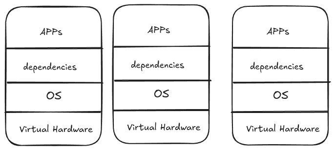
VMs solved hardware waste but created new problems at scale.
Every VM runs a complete operating system, if you have 1,000 VMs, you're running 1,000 complete operating systems, each consuming 2-4GB RAM, taking minutes to boot, and requiring constant maintenance.
Every operating system needs a license
Each VM's operating system needs monthly patches, security updates, backups, monitoring, and troubleshooting, at 1,000 VMs, you're maintaining 1,000 separate operating systems.
You need specialized VMware administrators, OS administrators for each type of VM, network virtualization experts, and storage specialists, even with templates, deploying a new VM takes days because it requires coordination across multiple expert teams.
Container Architecture
If you notice in the previous image, we are repeating the OS. We just need to change the app and its requirements.
Think about it: an OS is just a kernel (for hardware recognition - the black screen that appears when you turn on the PC) and user space. For running applications, we don't need the full user space, we only need the kernel (for hardware access).
Another thing - the VMs are already installed on a real (physical) machine that already has a kernel, so why not just use it? If we could use the host's kernel and get rid of the OS for each VM, we'd solve half the problem. This is one of the main ideas behind containers.
How can we do this? First, remember that the Linux kernel is the same everywhere in the world - what makes distributions different is the user space. Start with the kernel, add some tools and configurations, you get Debian. Add different tools, you get Ubuntu. It's always: kernel + different stuff on top = different distributions.
How do containers achieve this idea? By using layers. Think of it like a cake:
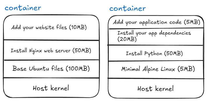
You can stop at any layer! Layer 1 alone (just the base OS files) is a valid container - yes, you can have a "container of an OS", but remember it's not a full OS, just the user space files without a kernel. Each additional layer adds something specific you need.
After you finish building these layers, you can save the complete stack as a template, this template is called an image. When you run an image, it becomes a running container.
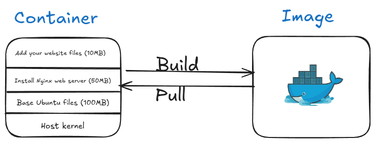
Remember, we don't care about the OS - Windows, Linux, macOS - they all have kernels. If your app needs Linux-specific tools or Windows-specific tools, you can add just those specific components in a layer and continue building. This reduces dependencies dramatically.
The idea is: start from the kernel and build up only what you need. But how exactly does this work?
The Linux Magic: cgroups and namespaces
Containers utilize Linux kernel features, specifically cgroups and namespaces.
cgroups (control groups): It controls how much CPU, memory, and disk a process can use.
Example:
- Process A: Use maximum 2 CPU cores and 4GB RAM
- Process B: Use maximum 1 CPU core and 2GB RAM
- Container = cgroups ensures Process A can't steal resources from Process B
namespaces: These manage process isolation and hierarchy, they make processes think they're alone on the system.
Example: Process tree isolation
Host System:
├── Process 1 (PID 1)
├── Process 2 (PID 2)
└── Process 3 (PID 3)
Inside Container (namespace):
└── Process 1 (thinks it's PID 1, but it's actually PID 453 on host)
└── Process 2 (thinks it's PID 2, but it's actually PID 454 on host)
The container's processes think they're the only processes on the system, completely unaware of other containers or host processes.
Containers = cgroups + namespaces + layers
If you think about it, cgroups + namespaces = container isolation. You start with one process, isolated in its own namespace with resource limits from cgroups. From that process, you install specific libraries, then Python, then pip install your dependencies, and each step is a layer.
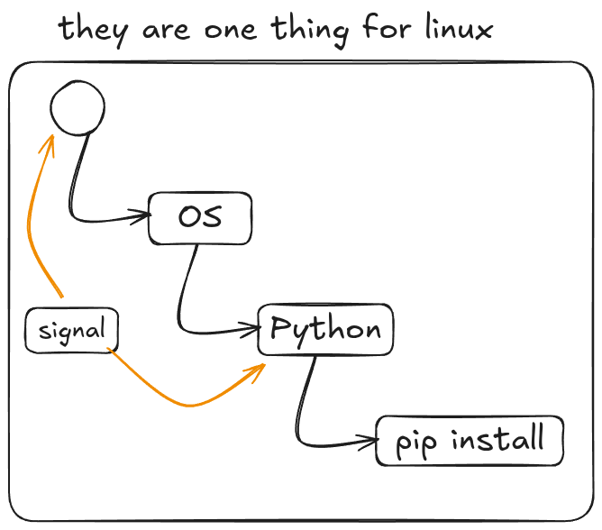
You can even utilize the same idea of Unix signals to control containers, and send SIGTERM to stop a process, and by extension, stop the entire container.
Because namespaces and cgroups are built into the Linux kernel, we only need the kernel, nothing else! No full operating system required.
The Tool: Docker
There are many technologies that achieve containerization (rkt, Podman, containerd), but the most famous one is made by Docker Inc. The software? They called it "Docker."
Yeah, super creative naming there, folks. :)
![]()
If you install Docker on Windows, you are actually installing Docker Desktop, which creates a lightweight virtual machine behind the scenes. Inside that VM, Docker runs a Linux environment, and your Linux containers run there.
If you want to run Windows containers, Docker Desktop can switch to Windows container mode, but those require the Windows kernel and cannot run inside the Linux VM.
Same for macOS.
If you install Docker on Linux, there is no virtual machine involved. You simply get the tools to create and run containers directly
Install Docker
For Windows of macOS see see: Overview of Docker Desktop.
If you are Ubuntu run these commands:
curl -fsSL https://get.docker.com -o get-docker.sh
Then
sudo sh ./get-docker.sh --dry-run
Then run to verify:
sudo docker info
If writing sudo everytime is annoying, then you need to yourself(the name of the user) to the docker group and then restart your machine:
Run the following with replacing mahmoudxyz with your username:
sudo usermod -aG docker mahmoudxyz
After you restart your PC, you will not need to use sudo again before docker.
Basic Docker Commands
Let's start with a simple command:
docker run -it python
This command creates and starts a container (a shortcut for docker create + docker start). The -i flag keeps STDIN open (interactive), and -t allocates a terminal (TTY).
Another useful thing about docker run is that if you don’t have the image locally, Docker will automatically pull it from Docker Hub.
The output of this command shows some downloads and other logs, but the most important part is something like:
Digest: sha256:[text here]
This string can also serve as your image ID.
After the download finishes, Docker will directly open the Python interactive mode:
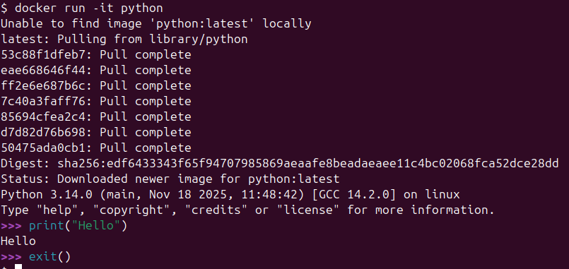
You can write Python code here, but if you exit Python, the entire container stops. This illustrates an important concept: a container is designed to run a single process. Once that process ends, the container itself ends.
| Command | Description | Example |
|---|---|---|
docker pull | Downloads an image from Docker Hub (or another registry) | docker pull fedora |
docker create | Creates a container from an image without starting it | docker create fedora |
docker run | Creates and starts a container (shortcut for create + start) | docker run fedora |
docker ps | Lists running containers | docker ps |
docker ps -a | Lists all containers (stopped + running) | docker ps -a |
docker images | Shows all downloaded images | docker images |
Useful Flags
| Flag | Meaning | Example |
|---|---|---|
-i | Keep STDIN open (interactive) | docker run -i fedora |
-t | Allocate a TTY (terminal) | docker run -t fedora |
-it | Interactive + TTY → lets you use the container shell | docker run -it fedora bash |
ls (in Docker context) | Used inside container to list files (Linux command) | docker run -it ubuntu ls |
To remove a container, use:
docker rm <container_id_or_name>
You can only remove stopped containers. If a container is running, you need to stop it first with:
docker stop <container_id_or_name>
Port Forwarding
When you run a container that exposes a service (like a web server), you often want to access it from your host machine. Docker allows this using the -p flag:
docker run -p <host_port>:<container_port> <image>
Example:
docker run -p 8080:80 nginx
- 8080 → the port on your host machine
- 80 → the port inside the container that Nginx listens on
Now, you can open your browser and visit: http://localhost:8080 …and you’ll see the Nginx welcome page.
Docker Networks (in nutshell)
Docker containers are isolated by default. Each container has its own network stack and cannot automatically see or communicate with other containers unless you connect them.
A Docker network allows containers to:
- Communicate with each other using container names instead of IPs.
- Avoid port conflicts and isolate traffic from the host or other containers.
- Use DNS resolution inside the network (so container1 can reach container2 by name).
Default Networks
Docker automatically creates a few networks:
- bridge → the default network for standalone containers.
- host → containers share the host’s network.
- none → containers have no network
If you want multiple containers (e.g., Jupyter + database) to talk to each other safely and easily, it’s best to create a custom network like bdb-net.
Example:
docker network create bdb-net
Jupyter Docker
Jupyter Notebook can easily run inside a Docker container, which helps avoid installing Python and packages locally.
Don't forget to create the network first:
docker network create bdb-net
docker run -d --rm --name my_jupyter --mount src=bdb_data,dst=/home/jovyan -p 127.0.0.1:8888:8888 --network bdb-net -e JUPYTER_ENABLE_LAB=yes -e JUPYTER_TOKEN="bdb_password" --user root -e CHOWN_HOME=yes -e CHOWN_HOME_OPTS="-R" jupyter/datascience-notebook
Flags and options:
| Option | Meaning |
|---|---|
-d | Run container in detached mode (in the background) |
--rm | Automatically remove container when it stops |
--name my_jupyter | Assign a custom name to the container |
--mount src=bdb_data,dst=/home/jovyan | Mount local volume bdb_data to /home/jovyan inside container |
-p 127.0.0.1:8888:8888 | Forward host localhost port 8888 to container port 8888 |
--network bdb-net | Connect container to Docker network bdb-net |
-e JUPYTER_ENABLE_LAB=yes | Start Jupyter Lab instead of classic Notebook |
-e JUPYTER_TOKEN="bdb_password" | Set a token/password for access |
--user root | Run container as root user (needed for certain permissions) |
-e CHOWN_HOME=yes -e CHOWN_HOME_OPTS="-R" | Change ownership of home directory to user inside container |
jupyter/datascience-notebook | The Docker image containing Python, Jupyter, and data science packages |
After running this, access Jupyter Lab at: http://127.0.0.1:8888. Use the token bdb_password to log in.
Topics (coming soon)
Docker engine architecture, docker image deep dives, container deep dives, Network
Pandas: Complete Notes
Setup
Every Pandas script starts with:
import pandas as pd
import numpy as np
pd and np are conventions. Everyone uses them.
Part 1: Series
A Series is a 1-dimensional array with labels (called an index).
s = pd.Series([1, 3, 5, np.nan, 6, 8])
print(s)
Output:
0 1.0
1 3.0
2 5.0
3 NaN
4 6.0
5 8.0
dtype: float64
The left column (0, 1, 2...) is the index. The right column is the values.
Accessing Index and Values Separately
print(s.index) # RangeIndex(start=0, stop=6, step=1)
print(s.values) # array([ 1., 3., 5., nan, 6., 8.])
Iterating Over a Series
# Just values
for i in s.values:
print(i)
# Both index and values
for i, v in s.items():
print(i, v)
Slicing a Series
Works like Python lists:
print(s[1:3]) # Elements at index 1 and 2 (3 is excluded)
Check for NaN
np.isnan(s[3]) # True
Custom Index
The index doesn't have to be integers:
students = pd.Series(
[28, 15, 30, 24, 10, 19],
index=['Lorenzo', 'Alessandra', 'Sofia', 'Giovanni', 'Matteo', 'Chiara']
)
print(students)
Output:
Lorenzo 28
Alessandra 15
Sofia 30
Giovanni 24
Matteo 10
Chiara 19
dtype: int64
Now you access by name:
print(students['Sofia']) # 30
Filtering a Series
print(students[students >= 18])
Output:
Lorenzo 28
Sofia 30
Giovanni 24
Chiara 19
dtype: int64
Creating Series from a Dictionary
capitals = pd.Series({
'Italy': 'Rome',
'Germany': 'Berlin',
'France': 'Paris',
'Spain': 'Madrid',
'Portugal': 'Lisbon'
})
Unlike regular Python dictionaries, Series support slicing:
print(capitals['France':'Portugal'])
Output:
France Paris
Spain Madrid
Portugal Lisbon
dtype: object
Convert Series to List
capitals.to_list() # ['Rome', 'Berlin', 'Paris', 'Madrid', 'Lisbon']
Part 2: DataFrames
A DataFrame is a 2-dimensional table. Each column is a Series.
Creating a DataFrame from Series
# First, create two Series with the same index
capitals = pd.Series({
'Italy': 'Rome',
'Germany': 'Berlin',
'France': 'Paris',
'Spain': 'Madrid',
'Portugal': 'Lisbon'
})
population = pd.Series({
'Italy': 58_800_000,
'Spain': 48_400_000,
'Germany': 84_400_000,
'Portugal': 10_400_000,
'France': 68_200_000
})
# Combine into DataFrame
countries = pd.DataFrame({'capitals': capitals, 'population': population})
print(countries)
Output:
capitals population
Italy Rome 58800000
Germany Berlin 84400000
France Paris 68200000
Spain Madrid 48400000
Portugal Lisbon 10400000
Creating a DataFrame from a Dictionary
df = pd.DataFrame({
'country': ['France', 'Germany', 'Italy', 'Portugal', 'Spain'],
'capital': ['Paris', 'Berlin', 'Rome', 'Lisbon', 'Madrid'],
'population': [68_200_000, 84_400_000, 58_800_000, 10_400_000, 48_400_000]
})
This creates an automatic numeric index (0, 1, 2...).
DataFrame Properties
print(countries.index) # Index(['Italy', 'Germany', 'France', 'Spain', 'Portugal'])
print(countries.columns) # Index(['capitals', 'population'])
print(countries.shape) # (5, 2) → 5 rows, 2 columns
print(countries.size) # 10 → total elements
Accessing Columns
Two ways:
# Bracket notation
countries['population']
# Dot notation
countries.population
Both return a Series.
Accessing Multiple Columns
Use a list inside brackets:
countries[['capitals', 'population']] # Returns a DataFrame
Slicing Rows
countries['Italy':] # From Italy to the end
countries[0:3] # Rows 0, 1, 2
Filtering
countries[countries.population > 60_000_000]
Iterating Over a Single Column
for cap in countries['capitals']:
print(cap)
Convert DataFrame to Dictionary
countries.to_dict()
Part 3: Reading Files
CSV Files
df = pd.read_csv('covid19-sample.csv')
Excel Files
First install openpyxl (only once):
!pip install openpyxl
Then:
df = pd.read_excel('covid19-sample.xlsx')
Important: Excel reading is 500-1000x slower than CSV. Use CSV when possible.
Reading from a URL
df = pd.read_csv('https://github.com/dsalomoni/bdb-2024/raw/main/covid/covid19-sample.csv')
Reading Only Specific Columns
my_columns = ['country', 'weekly_count', 'year_week']
df = pd.read_csv('covid19-sample.csv', usecols=my_columns)
Part 4: Inspecting Data
First/Last Rows
df.head() # First 5 rows
df.head(10) # First 10 rows
df.tail(3) # Last 3 rows
Shape and Size
df.shape # (rows, columns) tuple
df.size # Total elements = rows × columns
Column Names
df.columns
Unique Values in a Column
df['indicator'].unique() # Array of unique values
df['indicator'].nunique() # Count of unique values
Part 5: Selecting and Slicing
By Row Number
df[3500:3504] # Rows 3500, 3501, 3502, 3503
df[777:778] # Just row 777
Specific Column from a Slice
df[777:778]['year_week']
# or
df[777:778].year_week
Multiple Columns
df.head()[['country', 'year_week']]
Using loc[]
Access rows by index label or by condition:
# By label
df.loc[19828]
# By condition
df.loc[df.weekly_count > 4500]
Part 6: Filtering with Conditions
Direct Filtering
df[df['grade'] > 27]
Multiple Conditions
# AND - use &
df[(df['grade'] > 27) & (df['age'] < 30)]
# OR - use |
df[(df['grade'] > 29) | (df['age'] > 30)]
Important: Wrap each condition in parentheses.
Using query() — The Better Way
df.query('country=="Italy" and indicator=="cases"')
With variables:
start_week = '2020-10'
end_week = '2021-48'
df.query('year_week >= @start_week and year_week <= @end_week')
Or using string formatting:
df.query('country=="Italy" and indicator=="cases" and year_week>="%s" and year_week<="%s"' % (start_week, end_week))
Part 7: iterrows() vs query()
The Slow Way: iterrows()
it_cases = dict()
for index, row in df.iterrows():
if row['country'] == 'Italy':
if row['indicator'] == 'cases':
week = row['year_week']
if (week >= start_week) and (week <= end_week):
it_cases[week] = row['weekly_count']
df2 = pd.DataFrame(list(it_cases.items()), columns=['week', 'cases'])
Time: ~1.52 seconds for 41,000 rows
The Fast Way: query()
df3 = df.query('country=="Italy" and indicator=="cases" and year_week>="%s" and year_week<="%s"' % (start_week, end_week))
Time: ~0.01 seconds
query() is about 150x faster than iterrows().
Part 8: Sorting
Sort a Series
series.sort_values() # Ascending
series.sort_values(ascending=False) # Descending
Sort a DataFrame
df.sort_values(by='quantity') # By one column
df.sort_values(by='quantity', ascending=False) # Descending
df.sort_values(by=['column1', 'column2']) # By multiple columns
Sort a Dictionary with Pandas
x = {'apple': 5, 'banana': 2, 'orange': 8, 'grape': 1}
series_x = pd.Series(x)
sorted_x = series_x.sort_values().to_dict()
# {'grape': 1, 'banana': 2, 'apple': 5, 'orange': 8}
Part 9: Common Functions
sum()
df['weekly_count'].sum()
describe()
Generates statistics for numerical columns:
df.describe()
Output includes: count, mean, std, min, 25%, 50%, 75%, max
nunique() and unique()
df['country'].nunique() # Number of unique values
df['country'].unique() # Array of unique values
mean() and median()
df['salary'].mean() # Average
df['salary'].median() # Middle value
When to use which:
- Mean: When data is symmetrically distributed, no outliers
- Median: When data has outliers or is skewed
Example:
Blood pressure readings: 142, 124, 121, 150, 215
Mean = (142+124+121+150+215)/5 = 150.4
Median = 142 (middle value when sorted: 121, 124, 142, 150, 215)
The 215 outlier pulls the mean up but doesn't affect the median.
Part 10: groupby()
Split data into groups, then apply a function.
Basic groupby
df_grouped = df.groupby('continent')
This returns a DataFrameGroupBy object. By itself, not useful. You need to apply a function:
df.groupby('continent').sum()
df.groupby('continent')['weekly_count'].mean()
df.groupby('continent')['weekly_count'].count()
Multiple Statistics with agg()
df.groupby('Agency')['Salary Range From'].agg(['mean', 'median'])
Group by Multiple Columns
df.groupby(['Agency', 'Posting Type'])['Salary Range From'].mean()
To prevent the grouped columns from becoming the index:
df.groupby(['Agency', 'Posting Type'], as_index=False)['Salary Range From'].mean()
Accessing Groups
grouped = df.groupby('continent')
# What groups exist?
grouped.groups.keys()
# Get one specific group
grouped.get_group('Oceania')
# How many unique countries in Oceania?
grouped.get_group('Oceania')['country'].nunique()
# Which countries?
grouped.get_group('Oceania')['country'].unique()
Sorting groupby Results
df.groupby('Agency')['# Of Positions'].count().sort_values(ascending=False).head(10)
Part 11: cut() — Binning Data
Convert continuous values into categories.
Basic Usage
df = pd.DataFrame({'age': [25, 30, 35, 40, 45, 50, 55, 60, 65]})
bins = [20, 40, 60, 80]
df['age_group'] = pd.cut(df['age'], bins)
Result:
age age_group
0 25 (20, 40]
1 30 (20, 40]
2 35 (20, 40]
3 40 (20, 40]
4 45 (40, 60]
...
With Labels
df['age_group'] = pd.cut(df['age'], bins, labels=['young', 'middle', 'old'])
Automatic Bins
pd.cut(df['Salary Range From'], bins=3, labels=['low', 'middle', 'high'])
Pandas automatically calculates the bin ranges.
Combining cut() with groupby()
# Add salary category column
jobs['salary_bin'] = pd.cut(jobs['Salary Range From'], bins=3, labels=['low', 'middle', 'high'])
# Now group by it
jobs.groupby('salary_bin')['Salary Range From'].count()
Part 12: Data Cleaning
Removing Duplicates
# Remove duplicate rows (all columns must match)
df.drop_duplicates(inplace=True)
# Remove duplicates based on specific column
df.drop_duplicates(subset=['B'], inplace=True)
Handling Missing Values (NaN)
Option 1: Fill with a value
# Fill with mean
df['A'].fillna(df['A'].mean(), inplace=True)
# Fill with median
df['B'].fillna(df['B'].median(), inplace=True)
Option 2: Drop rows with NaN
df.dropna() # Drop any row with NaN
df.dropna(subset=['grade']) # Only if specific column is NaN
Part 13: Data Scaling
When columns have very different scales (e.g., age: 20-60, salary: 50000-200000), analysis and visualization become difficult.
Standardization (StandardScaler)
Transforms data to have mean = 0 and standard deviation = 1.
from sklearn.preprocessing import StandardScaler
df_unscaled = pd.DataFrame({'A': [1, 3, 2, 2, 1], 'B': [65, 130, 80, 70, 50]})
scaler = StandardScaler()
df_scaled = scaler.fit_transform(df_unscaled)
df_scaled = pd.DataFrame(df_scaled, columns=df_unscaled.columns)
When to use: Data follows a Gaussian (bell-shaped) distribution.
Normalization (MinMaxScaler)
Transforms data to range [0, 1].
from sklearn.preprocessing import MinMaxScaler
scaler = MinMaxScaler()
df_scaled = scaler.fit_transform(df_unscaled)
df_scaled = pd.DataFrame(df_scaled, columns=df_unscaled.columns)
When to use: Distribution is unknown or not Gaussian.
Warning: Normalization is more sensitive to outliers than standardization.
Part 14: Plotting
Basic Syntax
df.plot(x='column_x', y='column_y', kind='line')
Plot Types
| kind= | Plot Type |
|---|---|
'line' | Line plot |
'bar' | Bar chart |
'barh' | Horizontal bar |
'pie' | Pie chart |
'scatter' | Scatter plot |
'hist' | Histogram |
Examples
# Bar plot
df.plot(x='name', y='age', kind='bar', title='Ages')
# Line plot
df.plot(x='month', y='sales', kind='line', title='Monthly Sales')
# With more options
df.plot(kind='bar', ylabel='Total cases', title='COVID-19', grid=True, logy=True)
Plotting Two DataFrames Together
# Get axis from first plot
ax = df1.plot(kind='line', x='Month', title='Comparison')
# Add second plot to same axis
df2.plot(ax=ax, kind='line')
ax.set_xlabel('Month')
ax.set_ylabel('Sales')
ax.legend(['Vendor A', 'Vendor B'])
Part 15: Exporting Data
To CSV
df.to_csv('output.csv', index=False)
To Excel
df.to_excel('output.xlsx', index=False)
index=False prevents writing the row numbers as a column.
Part 16: Statistics Refresher
Variance and Standard Deviation
Variance (σ²): Average of squared differences from the mean.
$$\sigma^2 = \frac{\sum_{i=1}^{n}(x_i - \bar{x})^2}{n}$$
Standard Deviation (σ): Square root of variance.
$$\sigma = \sqrt{\sigma^2}$$
Why use standard deviation instead of variance?
- Variance has squared units (meters² if data is in meters)
- Standard deviation has the same units as the original data
- Standard deviation is more interpretable
Gaussian Distribution
A bell-shaped curve where:
- Mean, median, and mode are equal (at the center)
- ~68% of data falls within 1 standard deviation of the mean
- ~95% within 2 standard deviations
- ~99.7% within 3 standard deviations
Quick Reference
Reading
pd.read_csv('file.csv')
pd.read_csv('file.csv', usecols=['col1', 'col2'])
pd.read_excel('file.xlsx')
Inspecting
df.head(), df.tail()
df.shape, df.size, df.columns
df.describe()
df['col'].unique(), df['col'].nunique()
Selecting
df['col'] # Single column (Series)
df[['col1', 'col2']] # Multiple columns (DataFrame)
df[0:5] # Rows 0-4
df.loc[df['col'] > x] # By condition
df.query('col > x') # By condition (faster)
Cleaning
df.dropna()
df.fillna(value)
df.drop_duplicates()
Aggregating
df['col'].sum(), .mean(), .median(), .std(), .count()
df.groupby('col')['val'].mean()
df.groupby('col')['val'].agg(['mean', 'median', 'count'])
Sorting
df.sort_values(by='col')
df.sort_values(by='col', ascending=False)
Exporting
df.to_csv('out.csv', index=False)
df.to_excel('out.xlsx', index=False)
Performance Summary
| Operation | Speed |
|---|---|
read_csv() | Fast |
read_excel() | 500-1000x slower |
query() | Fast |
df[condition] | Fast |
iterrows() | ~150x slower than query() |
Rule: Avoid iterrows() on large datasets. Use query() or boolean indexing instead.
Introduction to Databases
A database (DB) is an organized collection of structured data stored electronically in a computer system, managed by a Database Management System (DBMS).
Let's Invent Database
Alright, so imagine you're building a movie collection app with Python. At first, you might think "I'll just use files!"
You create a file for each movie - titanic.txt, inception.txt, and so on. Inside each file, you write the title, director, year, rating. Simple enough!
But then problems start piling up. You want to find all movies from 2010? Now you're writing Python code to open every single file, read it, parse it, check the year. Slow and messy.
Your friend wants to update a movie's rating while you're reading it? Boom! File corruption or lost data because two programs can't safely write to the same file simultaneously.
You want to find all movies directed by Nolan AND released after 2010? Now your Python script is getting complex, looping through thousands of files, filtering multiple conditions.
What if the power goes out mid-write? Half-updated file, corrupted data.
This is where you start thinking, "there has to be a better way!" What if instead of scattered files, we had one organized system that could handle all this? A system designed from the ground up for concurrent access, fast searching, data integrity, and complex queries. That's the core idea behind what we'd call a database.
Database Management System
So you've realized you need a better system. Enter the DBMS, the Database Management System.
Instead of your Python code directly wrestling with files, the DBMS handles all the heavy lifting, managing storage, handling concurrent users, ensuring data doesn't get corrupted, and executing queries efficiently.
But here's the key question: how should we actually structure this data?
This is where the data model comes in. It's your blueprint for organizing information. For movies, you might think: "Every movie has attributes: title, director, year, rating." That's a relational model thinking, data organized in tables with rows and columns, like a spreadsheet but much more powerful.
Relational Model - Tables:
| movie_id | title | director | year | rating |
|---|---|---|---|---|
| 1 | Inception | Nolan | 2010 | 8.8 |
| 2 | Titanic | Cameron | 1997 | 7.9 |
| 3 | Interstellar | Nolan | 2014 | 8.7 |
Or maybe you think: "Movies are connected, directors make movies, actors star in them, movies belong to genres." That's more of a graph model, focusing on relationships between entities.
Graph Model - Nodes and Relationships:
(Movie: Inception)
|
|--[DIRECTED_BY]--> (Director: Nolan)
|
|--[RELEASED_IN]--> (Year: 2010)
|
|--[HAS_RATING]--> (Rating: 8.8)
(Movie: Interstellar)
|
|--[DIRECTED_BY]--> (Director: Nolan)
|
|--[RELEASED_IN]--> (Year: 2014)
The data model you choose shapes everything, how you store data, how you query it, how it performs. It's the fundamental architectural decision that defines your database.
What Is Schema ?
The schema is the blueprint (like class in Java or python) or structure of your database, it defines what can be stored and how it's organized, but not the actual data itself.
For our movie table, the schema would be:
Movies (
movie_id: INTEGER,
title: TEXT,
director: TEXT,
year: INTEGER,
rating: FLOAT
)
It specifies the table name, column names, and data types. It's like the architectural plan of a building, it shows the rooms and layout, but the furniture (actual data) comes later.
The schema enforces rules: you can't suddenly add a movie with a text value in the year field, or store a rating as a string. It keeps your data consistent and predictable.
Data Models
These are just example to know, but we will study only few, so it's ok if you they sounded complex, but they aren't.
Relational (SQL)
- Examples: PostgreSQL, MySQL, SQLite
- Use case: transactions. Need ACID guarantees, complex joins between related data.
Key-Value
- Examples: Redis, Memcached
- Use case: Session storage, user login tokens. Lightning-fast lookups by key, simple get/set operations.
Document/JSON (NoSQL)
- Examples: MongoDB, CouchDB
- Use case: Blog platform, each post is a JSON document with nested comments, tags, metadata. Flexible schema, easy to evolve.
Wide Column / Column Family
- Examples: Cassandra, HBase
- Use case: Time-series data like IoT sensors. Billions of writes per day, queried by device_id and timestamp range.
Array/Matrix/Vector
- Examples: PostgreSQL with pgvector, Pinecone, Weaviate
- Use case: AI embeddings for semantic search - store vectors representing documents, find similar items by vector distance.
Legacy Models:
- Hierarchical
- Network
- Semantic
- Entity-Relationship
The CAP Theorems
So you're building a distributed system. Maybe you've got servers in New York, London, and Tokyo because you want to be fancy and global. Everything's going great until someone asks you a simple question: "What happens when the network breaks?"
Welcome to the CAP theorem, where you learn that you can't have your cake, eat it too, and share it perfectly across three continents simultaneously.
The Three Musketeers (But Only Two Can Fight at Once)
CAP stands for Consistency, Availability, and Partition Tolerance. The theorem, courtesy of Eric Brewer in 2000, says you can only pick two out of three. It's like a cruel database version of "choose your fighter."
Consistency (C): Every node in your distributed system sees the same data at the same time. You read from Tokyo, you read from New York - same answer, guaranteed.
Availability (A): Every request gets a response, even if some nodes are down. The system never says "sorry, come back later."
Partition Tolerance (P): The system keeps working even when network connections between nodes fail. Because networks will fail - it's not if, it's when.
The "C" in CAP is NOT the same as the "C" in ACID! ACID consistency means your data follows all the rules (constraints, foreign keys). CAP consistency means all nodes agree on what the data is right now. Totally different beasts.
Why P Isn't Really Optional (Spoiler: Physics)
Here's the dirty secret: Partition Tolerance isn't actually optional in distributed systems. Network failures happen. Cables get cut. Routers die. Someone trips over the ethernet cord. Cosmic rays flip bits (yes, really).
If you're distributed across multiple machines, partitions will occur. So the real choice isn't CAP - it's really CP vs AP. You're choosing between Consistency and Availability when the network inevitably goes haywire.
If your "distributed system" is actually just one machine, congratulations! You can have CA because there's no network to partition. But then you're not really distributed, are you? This is why traditional RDBMS like PostgreSQL on a single server can give you strong consistency AND high availability.
CP: Consistency Over Availability
The Choice: "I'd rather return an error than return wrong data."
When a network partition happens, CP systems refuse to respond until they can guarantee you're getting consistent data. They basically say "I'm not going to lie to you, so I'm just going to shut up until I know the truth."
Examples: MongoDB (in default config), HBase, Redis (in certain modes), traditional SQL databases with synchronous replication.
When to choose CP:
- Banking and financial systems - you CANNOT have Bob's account showing different balances on different servers
- Inventory systems - overselling products because two datacenters disagree is bad for business
- Configuration management - if half your servers think feature X is on and half think it's off, chaos ensues
- Anything where stale data causes real problems, and it's better to show an error than a lie
Your bank's ATM won't let you withdraw money during a network partition because it can't verify your balance with the main server. Annoying? Yes. Better than letting you overdraw? Absolutely.
AP: Availability Over Consistency
The Choice: "I'd rather give you an answer (even if it might be stale) than no answer at all."
AP systems keep responding even during network partitions. They might give you slightly outdated data, but hey, at least they're talking to you! They eventually sync up when the network heals - this is called "eventual consistency."
Examples: Cassandra, DynamoDB, Riak, CouchDB, DNS (yes, the internet's phone book).
When to choose AP:
- Social media - if you see a slightly stale like count during a network issue, the world doesn't end
- Shopping cart systems - better to let users add items even if inventory count is slightly off, sort it out later
- Analytics dashboards - last hour's metrics are better than no metrics
- Caching layers - stale cache beats no cache
- Anything where availability matters more than perfect accuracy
Twitter/X during high traffic: you might see different follower counts on different servers for a few seconds. But the tweets keep flowing, the system stays up, and eventually everything syncs. For a social platform, staying online beats perfect consistency.
The "It Depends"
Here's where it gets interesting: modern systems often aren't pure CP or AP. They let you tune the trade-off!
Cassandra has a "consistency level" setting. Want CP behavior? Set it to QUORUM. Want AP? Set it to ONE. You're literally sliding the dial between consistency and availability based on what each query needs.
Different parts of your system can make different choices! Use CP for critical financial data, AP for user preferences and UI state. This is called "polyglot persistence" and it's how the big players actually do it.
The Plot Twist: PACELC
Just when you thought you understood CAP, along comes PACELC to ruin your day. It says: even when there's NO partition (normal operation), you still have to choose between Latency and Consistency.
Want every read to be perfectly consistent? You'll pay for it in latency because nodes have to coordinate. Want fast responses? Accept that reads might be slightly stale.
But that's a story for another day...
CAP isn't about right or wrong. It's about understanding trade-offs and making conscious choices based on your actual needs. The worst decision is not knowing you're making one at all.
TL;DR
You can't have perfect consistency, perfect availability, AND handle network partitions. Since partitions are inevitable in distributed systems, you're really choosing between CP (consistent but might go down) or AP (always available but might be stale).
Choose CP when wrong data is worse than no data. Choose AP when no data is worse than slightly outdated data.
Now go forth and distribute responsibly!
SQLite
What is a Relational Database?
A relational database organizes data into tables. Each table has:
- Rows (also called records) — individual entries
- Columns (also called fields) — attributes of each entry
Tables can be linked together through common fields. This is the "relational" part.
Part 1: Core Concepts
Schema
The schema is the structure definition of your database:
- Number of tables
- Column names and data types
- Constraints (what's allowed)
Critical: You must define the schema BEFORE you can store any data. This is a fixed structure — not flexible like a spreadsheet.
Primary Key
A column that uniquely identifies each row.
Rules:
- Only ONE primary key per table
- Values must be unique (no duplicates)
- Cannot be NULL
Example: Student ID, Order Number, ISBN
Foreign Key
A column that references a primary key in another table.
Rules:
- Can have multiple foreign keys in one table
- Values don't need to be unique
- Creates relationships between tables
Example: student_id in an Enrollments table references id in a Students table.
Why Use Multiple Tables?
Instead of repeating data:
# Bad: Student info repeated for each course
(1, 'Alice', 22, 'alice@unibo.it', 'BDB')
(2, 'Alice', 22, 'alice@unibo.it', 'BDP1') # Alice duplicated!
(3, 'Bob', 23, 'bob@unibo.it', 'BDB')
Use two linked tables:
Students:
(1, 'Alice', 22, 'alice@unibo.it')
(2, 'Bob', 23, 'bob@unibo.it')
Enrollments:
(1, 1, 'BDB') # student_id=1 (Alice)
(2, 1, 'BDP1') # student_id=1 (Alice)
(3, 2, 'BDB') # student_id=2 (Bob)
Benefits:
- No data duplication
- Update student info in one place
- Smaller storage
Part 2: ACID Properties
A transaction is a unit of work — a set of operations that must either all succeed or all fail.
ACID guarantees for transactions:
| Property | Meaning |
|---|---|
| Atomic | All operations complete, or none do |
| Consistent | Database goes from one valid state to another |
| Isolated | Transactions don't interfere with each other |
| Durable | Once committed, changes survive crashes/power failures |
Relational databases provide ACID compliance. This is why banks use them.
Part 3: SQLite
What is SQLite?
SQLite is a relational database that lives in a single file. No server needed.
It's everywhere:
- Every Android and iOS device
- Windows 10/11, macOS
- Firefox, Chrome, Safari
- Estimated 1 trillion+ SQLite databases in active use
SQLite vs Traditional Databases
| Traditional (PostgreSQL, MySQL) | SQLite |
|---|---|
| Separate server process | No server |
| Client connects via network | Direct file access |
| Multiple files | Single file |
| Complex setup | Zero configuration |
Python Support
Python has built-in SQLite support. No installation needed:
import sqlite3
Part 4: Connecting to SQLite
Basic Connection
import sqlite3 as sql
# Connect to database (creates file if it doesn't exist)
conn = sql.connect('my_database.db')
# Get a cursor (your pointer into the database)
cur = conn.cursor()
After this, you'll have a file called my_database.db in your directory.
In-Memory Database
For testing or temporary work:
conn = sql.connect(':memory:')
Fast, but everything is lost when you close Python.
What's a Cursor?
The cursor is how you execute commands and retrieve results. Think of it as your interface to the database.
cur.execute('SQL command here')
Part 5: Creating Tables
CREATE TABLE Syntax
cur.execute('''
CREATE TABLE Students (
id INTEGER PRIMARY KEY,
first_name TEXT NOT NULL,
last_name TEXT NOT NULL,
age INTEGER,
email TEXT NOT NULL UNIQUE
)
''')
Data Types
| Type | What it stores |
|---|---|
| INTEGER | Whole numbers |
| TEXT | Strings |
| REAL | Floating point numbers |
| BLOB | Binary data |
Constraints
| Constraint | Meaning |
|---|---|
| PRIMARY KEY | Unique identifier for each row |
| NOT NULL | Cannot be empty |
| UNIQUE | No duplicate values allowed |
The "Table Already Exists" Problem
If you run CREATE TABLE twice, you get an error.
Solution: Drop the table first if it exists.
cur.execute('DROP TABLE IF EXISTS Students')
cur.execute('''
CREATE TABLE Students (
id INTEGER PRIMARY KEY,
first_name TEXT NOT NULL,
last_name TEXT NOT NULL,
age INTEGER,
email TEXT NOT NULL UNIQUE
)
''')
Creating Tables with Foreign Keys
cur.execute('''DROP TABLE IF EXISTS Students''')
cur.execute('''
CREATE TABLE Students (
id INTEGER PRIMARY KEY,
first_name TEXT NOT NULL,
last_name TEXT NOT NULL,
age INTEGER,
email TEXT NOT NULL UNIQUE
)
''')
cur.execute('''DROP TABLE IF EXISTS Student_courses''')
cur.execute('''
CREATE TABLE Student_courses (
id INTEGER PRIMARY KEY,
student_id INTEGER NOT NULL,
course_id INTEGER,
course_name TEXT NOT NULL,
FOREIGN KEY(student_id) REFERENCES Students(id)
)
''')
conn.commit()
Part 6: Inserting Data
Single Row
cur.execute('''
INSERT INTO Students VALUES (1, 'John', 'Doe', 21, 'john@doe.com')
''')
What Happens If You Insert a Duplicate Primary Key?
cur.execute('''INSERT INTO Students VALUES (1, 'John', 'Doe', 21, 'john@doe.com')''')
cur.execute('''INSERT INTO Students VALUES (1, 'John', 'Doe', 21, 'john@doe.com')''')
# ERROR! id=1 already exists
Primary keys must be unique.
Multiple Rows with executemany()
the_students = (
(1, 'John', 'Doe', 21, 'john@doe.com'),
(2, 'Alice', 'Doe', 22, 'alice@doe.com'),
(3, 'Rose', 'Short', 21, 'rose@short.com')
)
cur.executemany('''INSERT INTO Students VALUES(?, ?, ?, ?, ?)''', the_students)
The ? Placeholders
Each ? gets replaced by one value from your tuple.
# 5 columns = 5 question marks
cur.executemany('''INSERT INTO Students VALUES(?, ?, ?, ?, ?)''', the_students)
Why use ? instead of string formatting?
- Cleaner code
- Prevents SQL injection attacks
- Handles escaping automatically
Part 7: The Commit Rule
Critical: Changes are NOT saved until you call commit().
cur.execute('INSERT INTO Students VALUES (4, "Diana", "Smith", 20, "diana@smith.com")')
# At this point, the data is only in memory
conn.commit() # NOW it's written to disk
If you close the connection without committing, all changes since the last commit are lost.
The Complete Pattern
# Make changes
cur.execute('INSERT ...')
cur.execute('UPDATE ...')
cur.execute('DELETE ...')
# Save to disk
conn.commit()
# Close when done
conn.close()
Part 8: Querying Data (SELECT)
Get All Rows
cur.execute('SELECT * FROM Students')
print(cur.fetchall())
Output:
[(1, 'John', 'Doe', 21, 'john@doe.com'),
(2, 'Alice', 'Doe', 22, 'alice@doe.com'),
(3, 'Rose', 'Short', 21, 'rose@short.com')]
fetchall() vs fetchone()
fetchall() returns a list of all rows:
cur.execute('SELECT * FROM Students')
all_rows = cur.fetchall() # List of tuples
fetchone() returns one row at a time:
cur.execute('SELECT * FROM Students')
first = cur.fetchone() # (1, 'John', 'Doe', 21, 'john@doe.com')
second = cur.fetchone() # (2, 'Alice', 'Doe', 22, 'alice@doe.com')
third = cur.fetchone() # (3, 'Rose', 'Short', 21, 'rose@short.com')
fourth = cur.fetchone() # None (no more rows)
Important: fetchall() Exhausts the Cursor
cur.execute('SELECT * FROM Students')
print(cur.fetchall()) # Returns all rows
print(cur.fetchall()) # Returns [] (empty list!)
Once you've fetched all rows, there's nothing left to fetch. You need to execute the query again.
Select Specific Columns
cur.execute('SELECT last_name, email FROM Students')
print(cur.fetchall())
# [('Doe', 'john@doe.com'), ('Doe', 'alice@doe.com'), ('Short', 'rose@short.com')]
Filter with WHERE
cur.execute('SELECT * FROM Students WHERE id=3')
print(cur.fetchall())
# [(3, 'Rose', 'Short', 21, 'rose@short.com')]
Pattern Matching with LIKE
# Emails ending with 'doe.com'
cur.execute("SELECT * FROM Students WHERE email LIKE '%doe.com'")
print(cur.fetchall())
# [(1, 'John', 'Doe', 21, 'john@doe.com'), (2, 'Alice', 'Doe', 22, 'alice@doe.com')]
Wildcards:
%— any sequence of characters (including none)_— exactly one character
Examples:
LIKE 'A%' # Starts with A
LIKE '%e' # Ends with e
LIKE '%li%' # Contains 'li'
LIKE '_ohn' # 4 characters ending in 'ohn' (John, Bohn, etc.)
Note: LIKE is case-insensitive in SQLite.
Part 9: Deleting Data
cur.execute('DELETE FROM Students WHERE id=1')
conn.commit()
Warning: Without WHERE, you delete everything:
cur.execute('DELETE FROM Students') # Deletes ALL rows!
Part 10: Error Handling
The Proper Pattern
import sqlite3 as sql
try:
conn = sql.connect('my_database.db')
cur = conn.cursor()
print("Connection successful")
# Your database operations here
cur.execute('SELECT * FROM Students')
print(cur.fetchall())
cur.close() # Close cursor to free memory
except sql.Error as error:
print("Error in SQLite:", error)
finally:
conn.close() # Always close connection, even if error occurred
Why use try/except/finally?
- Database operations can fail (file locked, disk full, etc.)
finallyensures connection is always closed- Prevents resource leaks
Part 11: Pandas Integration
This is where SQLite becomes really useful for data analysis.
Read SQLite into DataFrame
import pandas as pd
import sqlite3 as sql
conn = sql.connect('gubbio_env_2018.sqlite')
df = pd.read_sql_query('SELECT * FROM gubbio', conn)
conn.close()
Now you have a DataFrame with all the Pandas functionality.
df.head()
df.info()
df.describe()
Filter in SQL vs Filter in Pandas
Option 1: Filter in SQL (better for large databases)
df = pd.read_sql_query('SELECT * FROM gubbio WHERE NO2 > 50', conn)
Only matching rows are loaded into memory.
Option 2: Load all, filter in Pandas
df = pd.read_sql_query('SELECT * FROM gubbio', conn)
df_filtered = df[df['NO2'] > 50]
Loads everything, then filters.
Use SQL filtering when:
- Database is large
- You only need a small subset
Use Pandas filtering when:
- Data fits in memory
- You need multiple different analyses
Write DataFrame to SQLite
conn = sql.connect('output.sqlite')
df.to_sql('table_name', conn, if_exists='replace')
conn.close()
if_exists options:
'fail'— raise error if table exists (default)'replace'— drop table and recreate'append'— add rows to existing table
Part 12: Data Cleaning Example (Gubbio Dataset)
The Dataset
Environmental monitoring data from Gubbio, Italy (2018):
- Columns: year, month, day, hour, NO2, O3, PM10, PM25
- Values are in µg/m³
- Problem: Missing/invalid readings are coded as
-999
The Problem with -999 Values
df = pd.read_sql_query('SELECT * FROM gubbio', conn)
print(df['NO2'].mean()) # Wrong! Includes -999 values
The -999 values will drastically lower your mean.
Solution 1: Replace with 0 (for visualization only)
df.loc[df.NO2 < 0, 'NO2'] = 0
df.loc[df.O3 < 0, 'O3'] = 0
df.loc[df.PM10 < 0, 'PM10'] = 0
df.loc[df.PM25 < 0, 'PM25'] = 0
Good for plotting (no negative spikes), but bad for statistics — zeros still affect the mean.
Solution 2: Replace with NaN (for analysis)
import numpy as np
df.loc[df.NO2 < 0, 'NO2'] = np.nan
df.loc[df.O3 < 0, 'O3'] = np.nan
df.loc[df.PM10 < 0, 'PM10'] = np.nan
df.loc[df.PM25 < 0, 'PM25'] = np.nan
This is the correct approach. Pandas ignores NaN in calculations:
df['NO2'].mean() # Calculates mean of valid values only
Using loc[] to Find and Modify
Find rows matching condition:
# All rows where NO2 is negative
print(df.loc[df.NO2 < 0])
# Just the NO2 column where NO2 is negative
print(df.loc[df.NO2 < 0, 'NO2'])
Modify matching rows:
df.loc[df.NO2 < 0, 'NO2'] = np.nan
This reads: "For rows where NO2 < 0, set the NO2 column to NaN."
Part 13: DateTime Handling
Creating DateTime from Components
The Gubbio dataset has separate year, month, day, hour columns. Combine them:
df['timerep'] = pd.to_datetime(df[['year', 'month', 'day', 'hour']])
Result: A proper datetime column like 2018-01-01 00:00:00.
Setting DateTime as Index
df.set_index('timerep', inplace=True)
Now you can do time-based operations.
Check the Result
df.info()
You'll see DatetimeIndex instead of RangeIndex.
Part 14: Resampling (Time Aggregation)
What is Resampling?
Converting from higher frequency (hourly) to lower frequency (daily, monthly, yearly).
Basic Syntax
df.resample('D').mean() # Daily mean
df.resample('M').mean() # Monthly mean
df.resample('A').mean() # Annual mean
Resample Codes
| Code | Frequency |
|---|---|
| 'H' | Hourly |
| 'D' | Daily |
| 'W' | Weekly |
| 'M' | Monthly |
| 'A' | Annual/Yearly |
Examples
Daily mean of PM10, PM25, NO2:
df.resample('D').mean()[['PM10', 'PM25', 'NO2']]
Yearly mean:
df.resample('A').mean()[['PM10', 'PM25']]
Combining Resample with Query
Find days where PM10 exceeded 50 µg/m³ (WHO 24-hour limit):
df.resample('D').mean().query('PM10 > 50')[['PM10']]
This:
- Resamples to daily
- Computes the mean
- Filters to days where PM10 > 50
- Shows only the PM10 column
Find days where PM2.5 exceeded 24 µg/m³:
df.resample('D').mean().query('PM25 > 24')[['PM25']]
WHO Air Quality Limits
| Pollutant | Annual Limit | 24-Hour Limit |
|---|---|---|
| PM2.5 | 10 µg/m³ | 24 µg/m³ |
| PM10 | 20 µg/m³ | 50 µg/m³ |
Part 15: Saving and Loading with DateTime Index
The Problem
When you save a DataFrame with a datetime index to SQLite and read it back, the index might not be preserved correctly.
Wrong Way
# Save
df.to_sql('gubbio', conn, if_exists='replace')
# Load
df2 = pd.read_sql('SELECT * FROM gubbio', conn)
df2.plot(y=['NO2']) # X-axis is wrong!
Correct Way: Preserve the Index
Saving:
df.to_sql('gubbio', conn, if_exists='replace', index=True, index_label='timerep')
Loading:
df2 = pd.read_sql('SELECT * FROM gubbio', conn, index_col='timerep', parse_dates=['timerep'])
Parameters:
index=True— save the index as a columnindex_label='timerep'— name the index columnindex_col='timerep'— use this column as index when loadingparse_dates=['timerep']— parse as datetime
Part 16: Complete Workflow
Typical pattern: Load → Clean → Analyze → Save
import pandas as pd
import sqlite3 as sql
import numpy as np
# 1. Connect and load
conn = sql.connect('gubbio_env_2018.sqlite')
df = pd.read_sql_query('SELECT * FROM gubbio', conn)
# 2. Clean bad values (replace -999 with NaN)
df.loc[df.NO2 < 0, 'NO2'] = np.nan
df.loc[df.O3 < 0, 'O3'] = np.nan
df.loc[df.PM10 < 0, 'PM10'] = np.nan
df.loc[df.PM25 < 0, 'PM25'] = np.nan
# 3. Create datetime index
df['timerep'] = pd.to_datetime(df[['year', 'month', 'day', 'hour']])
df.set_index('timerep', inplace=True)
# 4. Analyze
# Daily averages
daily = df.resample('D').mean()[['PM10', 'PM25', 'NO2']]
# Days exceeding WHO PM10 limit
bad_pm10_days = df.resample('D').mean().query('PM10 > 50')[['PM10']]
print(f"Days PM10 > 50: {len(bad_pm10_days)}")
# Yearly average
yearly = df.resample('A').mean()[['PM10', 'PM25']]
print(yearly)
# 5. Plot
df.plot(y=['NO2'])
df.plot(y=['O3'])
# 6. Save results
df.to_sql('gubbio_clean', conn, if_exists='replace', index=True, index_label='timerep')
# 7. Close
conn.close()
SQL Commands Summary
| Command | Purpose | Example |
|---|---|---|
| CREATE TABLE | Define schema | CREATE TABLE Students (id INTEGER PRIMARY KEY, name TEXT) |
| DROP TABLE | Delete table | DROP TABLE IF EXISTS Students |
| INSERT INTO | Add rows | INSERT INTO Students VALUES (1, 'Alice') |
| SELECT | Query data | SELECT * FROM Students WHERE age > 20 |
| DELETE | Remove rows | DELETE FROM Students WHERE id = 1 |
| LIKE | Pattern match | SELECT * FROM Students WHERE name LIKE 'A%' |
Python SQLite Summary
| Operation | Code |
|---|---|
| Connect | conn = sql.connect('file.db') |
| Get cursor | cur = conn.cursor() |
| Execute | cur.execute('SQL') |
| Execute many | cur.executemany('SQL', list_of_tuples) |
| Fetch one | cur.fetchone() |
| Fetch all | cur.fetchall() |
| Save changes | conn.commit() |
| Close cursor | cur.close() |
| Close connection | conn.close() |
Pandas + SQLite Summary
| Operation | Code |
|---|---|
| Read | pd.read_sql_query('SELECT...', conn) |
| Read with index | pd.read_sql_query('...', conn, index_col='col', parse_dates=['col']) |
| Write | df.to_sql('table', conn, if_exists='replace') |
| Write with index | df.to_sql('table', conn, if_exists='replace', index=True, index_label='name') |
Common Mistakes
| Mistake | Problem | Fix |
|---|---|---|
Forgot conn.commit() | Changes not saved | Always commit after INSERT/UPDATE/DELETE |
Using == in SQL | Syntax error | Use single = for equality |
| Replace -999 with 0 | Wrong statistics | Use np.nan instead |
DELETE FROM table without WHERE | Deletes everything | Always specify condition |
| CREATE TABLE twice | Error | Use DROP TABLE IF EXISTS first |
Wrong number of ? | Error | Must match column count |
| Not closing connection | Resource leak | Always conn.close() |
| fetchall() twice | Empty second result | Re-execute query or use fetchone() |
Quick Reference Card
import sqlite3 as sql
import pandas as pd
import numpy as np
# Connect
conn = sql.connect('database.db')
cur = conn.cursor()
# Create table
cur.execute('DROP TABLE IF EXISTS MyTable')
cur.execute('CREATE TABLE MyTable (id INTEGER PRIMARY KEY, value REAL)')
# Insert
cur.executemany('INSERT INTO MyTable VALUES (?, ?)', [(1, 10.5), (2, 20.3)])
conn.commit()
# Query
cur.execute('SELECT * FROM MyTable WHERE value > 15')
results = cur.fetchall()
# Load into Pandas
df = pd.read_sql_query('SELECT * FROM MyTable', conn)
# Clean data
df.loc[df.value < 0, 'value'] = np.nan
# Save back
df.to_sql('MyTable', conn, if_exists='replace', index=False)
# Close
conn.close()
ACID: The Database's Solemn Vow (NOT EXAM)
Picture this: You're transferring $500 from your savings to your checking account. The database deducts $500 from savings... and then the power goes out. Did the money vanish into the digital void? Did it get added to checking? Are you now $500 poorer for no reason?
This is the nightmare that keeps database architects up at night. And it's exactly why ACID exists.
ACID is a set of properties that guarantees your database transactions are reliable, even when the universe conspires against you. It stands for Atomicity, Consistency, Isolation, and Durability - which sounds like boring corporate jargon until you realize it's the difference between "my money's safe" and "WHERE DID MY MONEY GO?!"
A is for Atomicity: All or Nothing, Baby
Atomicity means a transaction is indivisible - it's an atom (get it?). Either the entire thing happens, or none of it does. No half-baked in-between states.
Back to our money transfer:
BEGIN TRANSACTION;
UPDATE accounts SET balance = balance - 500 WHERE account_id = 'savings';
UPDATE accounts SET balance = balance + 500 WHERE account_id = 'checking';
COMMIT;
If the power dies after the first UPDATE, atomicity guarantees that when the system comes back up, it's like that first UPDATE never happened. Your savings account still has the $500. The transaction either completes fully (both updates) or rolls back completely (neither update).
Ordering a pizza. Either you get the pizza AND they charge your card, or neither happens. You can't end up with "they charged me but I got no pizza" or "I got pizza but they forgot to charge me." Well, okay, in real life that sometimes happens. But in ACID databases? Never.
Atomicity doesn't mean fast or instant. It means indivisible. A transaction can take 10 seconds, but it's still atomic - either all 10 seconds of work commits, or none of it does.
C is for Consistency: Follow the Rules or Get Out
Consistency means your database moves from one valid state to another valid state. All your rules - constraints, triggers, cascades, foreign keys - must be satisfied before and after every transaction.
Let's say you have a rule: "Account balance cannot be negative." Consistency guarantees that no transaction can violate this, even temporarily during execution.
-- This has a constraint: balance >= 0
UPDATE accounts SET balance = balance - 1000 WHERE account_id = 'savings';
If your savings only has $500, this transaction will be rejected. The database won't let you break the rules, even for a nanosecond.
Remember: ACID consistency is about business rules and constraints within your database. CAP consistency (from the previous article) is about all servers in a distributed system agreeing on the same value. Same word, completely different meanings. Because computer science loves confusing us.
I is for Isolation: Mind Your Own Business
Isolation means concurrent transactions don't step on each other's toes. When multiple transactions run at the same time, they should behave as if they're running one after another, in some order.
Imagine two people trying to book the last seat on a flight at the exact same moment:
Transaction 1: Check if seats available → Yes → Book seat
Transaction 2: Check if seats available → Yes → Book seat
Without isolation, both might see "seats available" and both book the same seat. Chaos! Isolation prevents this by making sure transactions don't see each other's half-finished work.
Isolation actually has different levels (Read Uncommitted, Read Committed, Repeatable Read, Serializable). Stronger isolation = safer but slower. Weaker isolation = faster but riskier. Most databases default to something in the middle because perfect isolation is expensive.
The Classic Problem: Dirty Reads, Phantom Reads, and Other Horror Stories
Without proper isolation, you get gems like:
Dirty Read: You read data that another transaction hasn't committed yet. They roll back, and you read data that never actually existed. Spooky!
Non-Repeatable Read: You read a value, someone else changes it, you read it again in the same transaction and get a different answer. Identity crisis for data!
Phantom Read: You run a query that returns 5 rows. Run it again in the same transaction, now there are 6 rows because someone inserted data. Where did that 6th row come from? It's a phantom!
Two users book the same hotel room because both checked availability before either transaction committed. Isolation levels (like Serializable) prevent this by locking the relevant rows or using techniques like MVCC (Multi-Version Concurrency Control).
D is for Durability: Once Committed, Forever Committed
Durability means once a transaction is committed, it's permanent. Even if the server explodes, catches fire, and falls into the ocean immediately after, your committed data is safe.
How? Write-Ahead Logging (WAL), journaling, replication - databases use all kinds of tricks to write data to disk before saying "yep, it's committed!"
COMMIT; -- At this moment, the database promises your data is SAFE
-- Server can crash now, data is still there when it comes back up
When you COMMIT, the database doesn't just trust RAM. It writes to persistent storage (disk, SSD) and often waits for the OS to confirm the write completed. This is why commits can feel slow - durability isn't free, but it's worth every millisecond when disaster strikes.
When ACID Matters (Hint: More Than You Think)
Absolutely need ACID:
- Banking and financial systems - money doesn't just disappear or duplicate
- E-commerce - orders, payments, inventory must be consistent
- Medical records - patient data integrity is literally life-or-death
- Booking systems - double-booking is unacceptable
- Anything involving legal compliance or auditing
Maybe can relax ACID:
- Analytics dashboards - approximate counts are fine
- Social media likes - if a like gets lost in the noise, who cares?
- Caching layers - stale cache is better than no cache
- Logging systems - losing 0.01% of logs during a crash might be acceptable
"Our app is simple, we don't need all that ACID overhead!" - said every developer before they had to explain to their CEO why customer orders disappeared. Don't be that developer.
The Trade-off: ACID vs Performance
Here's the uncomfortable truth: ACID guarantees aren't free. They cost performance.
Ensuring atomicity? Needs transaction logs.
Enforcing consistency? Needs constraint checking.
Providing isolation? Needs locking or MVCC overhead.
Guaranteeing durability? Needs disk writes and fsyncs.
This is why NoSQL databases got popular in the early 2010s. They said "what if we... just didn't do all that?" and suddenly you could handle millions of writes per second. Of course, you also had data corruption, lost writes, and race conditions, but hey, it was fast!
MongoDB famously had a "durability" setting that was OFF by default for years. Your data wasn't actually safe after a commit unless you explicitly turned on write concerns. They fixed this eventually, but not before countless developers learned about durability the hard way.
Modern Databases: Having Your Cake and Eating It Too
The plot twist? Modern databases are getting really good at ACID without sacrificing too much performance:
- PostgreSQL uses MVCC (Multi-Version Concurrency Control) for high-performance isolation
- CockroachDB gives you ACID and horizontal scaling
- Google Spanner provides global ACID transactions across datacenters
The "NoSQL vs SQL" war has settled into "use the right tool for the job, and maybe that tool is a NewSQL database that gives you both."
Don't sacrifice ACID unless you have a specific, measured performance problem. Premature optimization killed more projects than slow databases ever did. Start with ACID, relax it only when you must.
TL;DR
ACID is your database's promise that your data is safe and correct:
- Atomicity: All or nothing - no half-done transactions
- Consistency: Rules are never broken - constraints always hold
- Isolation: Transactions don't interfere with each other
- Durability: Committed means forever - even through disasters
Yes, it costs performance. No, you probably shouldn't skip it unless you really, REALLY know what you're doing and have a very good reason.
Your future self (and your CEO) will thank you when the server crashes and your data is still intact.
Database Management System Architecture [NOT EXAM]
So you've got data. Lots of it. And you need to store it, query it, update it, and make sure it doesn't explode when a thousand users hit it simultaneously. Enter the DBMS - the unsung hero working behind the scenes while you're busy writing SELECT * FROM users.
But what actually happens when you fire off that query? What's going on in the engine room? Let's pop the hood and see how these beautiful machines work.
The Big Picture: Layers Upon Layers
A DBMS is like an onion - layers upon layers, and sometimes it makes you cry when you dig too deep. But unlike an onion, each layer has a specific job and they all work together in harmony (most of the time).
Think of it as a restaurant:
- Query Interface: The waiter taking your order
- Query Processor: The chef figuring out how to make your dish
- Storage Manager: The kitchen staff actually cooking and storing ingredients
- Transaction Manager: The manager making sure orders don't get mixed up
- Disk Storage: The pantry and freezer where everything lives
Let's break down each component and see what it actually does.
1. Query Interface: "Hello, How Can I Help You?"
This is where you interact with the database. It's the friendly face (or command line) that accepts your SQL queries, API calls, or whatever language your DBMS speaks.
Components:
- SQL Parser: Takes your SQL string and turns it into something the computer understands
- DDL Compiler: Handles schema definitions (CREATE TABLE, ALTER TABLE)
- DML Compiler: Handles data manipulation (SELECT, INSERT, UPDATE, DELETE)
SELECT * FROM users WHERE age > 18;
The parser looks at this and thinks: "Okay, they want data. From the 'users' table. With a condition. Got it." Then it passes this understanding down the chain.
When you write terrible SQL with syntax errors, this is where it gets caught. The parser is that friend who tells you "that's not how you spell SELECT" before you embarrass yourself further.
2. Query Processor: The Brain of the Operation
This is where the magic happens. Your query might say "give me all users over 18," but HOW should the database do that? Scan every single row? Use an index? Check the age column first or last? The query processor figures all this out.
Key Components:
Query Optimizer
The optimizer is basically an AI that's been doing its job since the 1970s. It looks at your query and generates multiple execution plans, then picks the best one based on statistics about your data.
SELECT u.name, o.total
FROM users u
JOIN orders o ON u.id = o.user_id
WHERE u.country = 'Italy';
The optimizer thinks: "Should I find Italian users first, then join orders? Or scan orders first? How many Italian users are there? Is there an index on country? On user_id?" It runs the math and picks the fastest path.
This is why adding an index can make queries 1000x faster. The optimizer sees the index and thinks "oh perfect, I can use that instead of scanning millions of rows!" Same query, completely different execution plan.
Query Execution Engine
Once the optimizer picks a plan, the execution engine actually runs it. It's the worker bee that fetches data, applies filters, joins tables, and assembles your result set.
Most databases let you see the query plan with EXPLAIN or EXPLAIN ANALYZE. If your query is slow, this is your first stop. The optimizer shows you exactly what it's doing, and often you'll spot the problem immediately - like a missing index or an accidental full table scan.
3. Transaction Manager: Keeping the Peace
Remember ACID? This is where it happens. The transaction manager makes sure multiple users can work with the database simultaneously without chaos erupting.
Key Responsibilities:
Concurrency Control
Prevents the classic problems: two people trying to buy the last concert ticket, or withdrawing money from the same account simultaneously. Uses techniques like:
- Locking: "Sorry, someone else is using this row right now, wait your turn"
- MVCC (Multi-Version Concurrency Control): "Here's your own snapshot of the data, everyone gets their own version"
- Timestamp Ordering: "We'll execute transactions in timestamp order, nice and orderly"
Recovery Manager
When things go wrong (power outage, crash, cosmic ray), this component brings the database back to a consistent state. It uses:
- Write-Ahead Logging (WAL): Write to the log before writing to the database, so you can replay or undo operations
- Checkpoints: Periodic snapshots so recovery doesn't have to replay the entire history since the Big Bang
- Rollback: Undo incomplete transactions
- Roll-forward: Redo committed transactions that didn't make it to disk
When you COMMIT, the database doesn't just write to memory and call it a day. It writes to the WAL, flushes to disk, and waits for confirmation. This is why durability costs performance - but it's also why your data survives disasters.
4. Storage Manager: Where Bytes Live
This layer manages the actual storage of data on disk (or SSD, or whatever physical medium you're using). It's the bridge between "logical" concepts like tables and rows, and "physical" reality like disk blocks and file pointers.
Components:
Buffer Manager
RAM is fast, disk is slow. The buffer manager keeps frequently accessed data in memory (the buffer pool) so queries don't have to hit disk constantly.
It's like keeping your favorite snacks on the counter instead of going to the store every time you're hungry.
When memory fills up, it uses replacement policies (LRU - Least Recently Used is popular) to decide what to kick out.
File Manager
Manages the actual files on disk. Tables aren't stored as neat CSV files - they're stored in complex structures optimized for different access patterns:
- Heap Files: Unordered collection of records, good for full table scans
- Sorted Files: Records sorted by some key, good for range queries
- Hash Files: Records distributed by hash function, good for exact-match lookups
- Clustered Files: Related records stored together, good for joins
Index Manager
Manages indexes - the phone book of your database. Instead of scanning every row to find what you want, indexes let you jump straight to the relevant data.
Common index types:
- B-Tree / B+Tree: Sorted tree structure, handles ranges beautifully
- Hash Index: Lightning fast for exact matches, useless for ranges
- Bitmap Index: Great for columns with few distinct values (like gender, status)
- Full-Text Index: Specialized for text search
Finding a user by ID without an index: scan 10 million rows, takes seconds.
Finding a user by ID with a B-tree index: traverse a tree with height ~4, takes milliseconds.
Same query, 1000x speed difference. Indexes are your friend!
5. The Disk Storage Layer: Ground Zero
At the bottom of it all, your data lives on physical storage. This layer deals with the gritty details:
- Blocks/Pages: Data is stored in fixed-size chunks (usually 4KB-16KB)
- Slotted Pages: How records fit inside blocks
- Free Space Management: Tracking which blocks have room for new data
- Data Compression: Squeezing more data into less space
Modern databases are incredibly clever here. They use techniques like:
- Column-oriented storage: Store columns separately for analytics workloads
- Compression: Save disk space and I/O bandwidth
- Partitioning: Split huge tables across multiple physical locations
- CPU Cache: ~1 nanosecond
- RAM: ~100 nanoseconds
- SSD: ~100 microseconds (1000x slower than RAM!)
- HDD: ~10 milliseconds (100,000x slower than RAM!)
This is why the buffer manager is so critical. Every disk access avoided is a massive win.
Architectural Patterns: Different Strokes for Different Folks
Not all DBMS architectures are the same. They evolved to solve different problems.
Centralized Architecture
Traditional, single-server setup. Everything lives on one machine.
Pros: Simple, full ACID guarantees, no network latency between components
Cons: Limited by one machine's resources, single point of failure
Example: PostgreSQL or MySQL on a single server
Client-Server Architecture
Clients connect to a central database server. Most common pattern today.
Pros: Centralized control, easier security, clients can be lightweight
Cons: Server can become a bottleneck
Example: Your web app connecting to a PostgreSQL server
Distributed Architecture
Data spread across multiple nodes, often in different locations.
Pros: Massive scalability, fault tolerance, can survive node failures
Cons: Complex, CAP theorem strikes, eventual consistency headaches
Example: Cassandra, MongoDB sharded clusters, CockroachDB
Parallel Architecture
Multiple processors/cores working on the same query simultaneously.
Types:
- Shared Memory: All processors share RAM and disk (symmetric multiprocessing)
- Shared Disk: Processors have their own memory but share disks
- Shared Nothing: Each processor has its own memory and disk (most scalable)
Example: Modern PostgreSQL can parallelize queries across cores
We went from centralized mainframes (1970s) → client-server (1990s) → distributed NoSQL (2000s) → distributed NewSQL (2010s). Each era solved the previous era's limitations while introducing new challenges.
Modern Twists: Cloud and Serverless
The cloud changed the game. Now we have:
Database-as-a-Service (DBaaS): Amazon RDS, Google Cloud SQL - you get a managed database without worrying about the infrastructure.
Serverless Databases: Aurora Serverless, Cosmos DB - database scales automatically, you pay per query.
Separation of Storage and Compute: Modern architectures split storage (S3, object storage) from compute (query engines). Scale them independently!
Traditional databases bundle everything together. Modern cloud databases separate concerns: storage is cheap and infinite (S3), compute is expensive and scales (EC2). Why pay for compute when you're not querying? This is the serverless revolution.
Putting It All Together: A Query's Journey
Let's trace what happens when you run a query:
SELECT name, email FROM users WHERE age > 25 ORDER BY name LIMIT 10;
- Query Interface: Parses the SQL, validates syntax
- Query Processor: Optimizer creates execution plan ("use age index, sort results, take first 10")
- Transaction Manager: Assigns a transaction ID, determines isolation level
- Storage Manager:
- Buffer manager checks if needed data is in memory
- If not, file manager reads from disk
- Index manager uses age index to find matching rows
- Execution Engine: Applies filter, sorts, limits results
- Transaction Manager: Commits transaction, releases locks
- Query Interface: Returns results to your application
All this happens in milliseconds. Databases are incredibly sophisticated machines!
Next time your query returns in 50ms, take a moment to appreciate the decades of computer science and engineering that made it possible. From parsing to optimization to disk I/O to lock management - it's a symphony of coordinated components.
TL;DR
A DBMS is a complex system with multiple layers:
- Query Interface: Takes your SQL and validates it
- Query Processor: Figures out the best way to execute your query
- Transaction Manager: Ensures ACID properties and handles concurrency
- Storage Manager: Manages buffer pool, files, and indexes
- Disk Storage: Where your data actually lives
Different architectures (centralized, distributed, parallel) trade off simplicity vs scalability vs consistency.
Modern databases are moving toward cloud-native, separation of storage and compute, and serverless models.
The next time you write SELECT *, remember: there's a whole orchestra playing in the background to make that query work.
Concurrency Control Theory -not for exam
Remember our ACID article? We talked about how databases promise to keep your data safe and correct. But there's a problem we glossed over: what happens when multiple transactions run at the same time?
Spoiler alert: chaos. Beautiful, fascinating, wallet-draining chaos.
The $25 That Vanished Into Thin Air
Let's start with a horror story. You've got $100 in your bank account. You try to pay for something that costs $25. Simple, right?
Read Balance: $100
Check if $100 > $25? ✓
Pay $25
New Balance: $75
Write Balance: $75
Works perfectly! Until the power goes out right after you read the balance but before you write it back. Now what? Did the payment go through? Is your money gone? This is where Atomicity saves you - either the entire transaction happens or none of it does.
But here's an even scarier scenario: What if TWO payments of $25 try to execute at the exact same time?
Transaction 1: Read Balance ($100) → Check funds → Pay $25
Transaction 2: Read Balance ($100) → Check funds → Pay $25
Transaction 1: Write Balance ($75)
Transaction 2: Write Balance ($75)
Both transactions read $100, both think they have enough money, both pay $25... and your final balance is $75 instead of $50. You just got a free $25! (Your bank is not happy.)
This is the nightmare that keeps database architects awake at night. And it's exactly why concurrency control exists.
These aren't theoretical problems. In 2012, Knight Capital lost $440 million in 45 minutes due to a race condition in their trading system. Concurrent transactions matter!
The Strawman Solution: Just Don't
The simplest solution? Don't allow concurrency at all. Execute one transaction at a time, in order, like a polite British queue.
Transaction 1 → Complete → Transaction 2 → Complete → Transaction 3 → ...
Before each transaction starts, copy the entire database to a new file. If it succeeds, overwrite the original. If it fails, delete the copy. Done!
This actually works! It's perfectly correct! It also has the performance of a potato.
Why? Because while one transaction is waiting for a slow disk read, every other transaction in the world is just... waiting. Doing nothing. Your expensive multi-core server is running one thing at a time like it's 1975.
We can do better.
The Goal: Having Your Cake and Eating It Too
What we actually want:
- Better utilization: Use all those CPU cores! Don't let them sit idle!
- Increased response times: When one transaction waits for I/O, let another one run
- Correctness: Don't lose money or corrupt data
- Fairness: Don't let one transaction starve forever
The challenge is allowing transactions to interleave their operations while still maintaining the illusion that they ran one at a time.
A schedule (interleaving of operations) is serializable if its result is equivalent to *some* serial execution of the transactions. We don't care which order, just that there exists *some* valid serial order that produces the same result.
The DBMS View: It's All About Reads and Writes
The database doesn't understand your application logic. It doesn't know you're transferring money or booking hotel rooms. All it sees is:
Transaction T1: R(A), W(A), R(B), W(B)
Transaction T2: R(A), W(A), R(B), W(B)
Where R = Read and W = Write. That's it. The DBMS's job is to interleave these operations in a way that doesn't break correctness.
The Classic Example: Interest vs Transfer
You've got two accounts, A and B, each with $1000. Two transactions run:
T1: Transfer $100 from A to B
A = A - 100 // A becomes $900
B = B + 100 // B becomes $1100
T2: Add 6% interest to both accounts
A = A * 1.06
B = B * 1.06
What should the final balance be? Well, A + B should equal $2120 (the original $2000 plus 6% interest).
Serial Execution: The Safe Path
If T1 runs completely before T2:
A = 1000 - 100 = 900
B = 1000 + 100 = 1100
Then apply interest:
A = 900 * 1.06 = 954
B = 1100 * 1.06 = 1166
Total: $2120 ✓
If T2 runs completely before T1:
A = 1000 * 1.06 = 1060
B = 1000 * 1.06 = 1060
Then transfer:
A = 1060 - 100 = 960
B = 1060 + 100 = 1160
Total: $2120 ✓
Both valid! Different final states, but both correct because A + B = $2120.
Good Interleaving: Still Correct
T1: A = A - 100 (A = 900)
T1: B = B + 100 (B = 1100)
T2: A = A * 1.06 (A = 954)
T2: B = B * 1.06 (B = 1166)
Total: $2120 ✓
This interleaving is equivalent to running T1 then T2 serially. We're good!
Bad Interleaving: Money Disappears
T1: A = A - 100 (A = 900)
T2: A = A * 1.06 (A = 1060) ← Used old value of A!
T2: B = B * 1.06 (B = 1060)
T1: B = B + 100 (B = 1160) ← Used old value of B!
Total: $2114 ✗
We lost $6! This schedule is NOT equivalent to any serial execution. It's incorrect.
T1 read A before T2 updated it, but T2 read B before T1 updated it. The transactions are interleaved in an inconsistent way - each transaction sees a mix of old and new values.
Conflicting Operations: The Root of All Evil
When do operations actually conflict? When they can cause problems if interleaved incorrectly?
Two operations conflict if:
- They're from different transactions
- They're on the same object (same data item)
- At least one is a write
This gives us three types of conflicts:
Read-Write Conflicts: The Unrepeatable Read
T1: R(A) → sees $10
T2: W(A) → writes $19
T1: R(A) → sees $19
T1 reads A twice in the same transaction and gets different values! The data changed underneath it. This is called an unrepeatable read.
Write-Read Conflicts: The Dirty Read
T1: W(A) → writes $12 (not committed yet)
T2: R(A) → reads $12
T2: W(A) → writes $14 (based on dirty data)
T2: COMMIT
T1: ROLLBACK ← Oh no!
T2 read data that T1 wrote but never committed. That data never "really existed" because T1 rolled back. T2 made decisions based on a lie. This is a dirty read.
You're booking the last seat on a flight. The reservation system reads "1 seat available" from a transaction that's updating inventory but hasn't committed. You book the seat. That transaction rolls back. Turns out there were actually 0 seats. Now you're stuck at the airport arguing with gate agents.
Write-Write Conflicts: The Lost Update
T1: W(A) → writes "Bob"
T2: W(A) → writes "Alice"
T2's write overwrites T1's write. If T1 hasn't committed yet, its update is lost. This is the lost update problem.
Conflict Serializability: The Practical Standard
Now we can formally define what makes a schedule acceptable. A schedule is conflict serializable if we can transform it into a serial schedule by swapping non-conflicting operations.
The Dependency Graph Trick
Here's a clever way to check if a schedule is conflict serializable:
- Draw one node for each transaction
- Draw an edge from Ti to Tj if Ti has an operation that conflicts with an operation in Tj, and Ti's operation comes first
- If the graph has a cycle, the schedule is NOT conflict serializable
Example: The Bad Schedule
T1: R(A), W(A), R(B), W(B)
T2: R(A), W(A), R(B), W(B)
With interleaving:
T1: R(A), W(A)
T2: R(A), W(A)
T2: R(B), W(B)
T1: R(B), W(B)
Dependency graph:
T1 → T2 (T1 writes A, T2 reads A - T1 must come first)
T2 → T1 (T2 writes B, T1 reads B - T2 must come first)
There's a cycle! T1 needs to come before T2 AND T2 needs to come before T1. Impossible! This schedule is not conflict serializable.
The dependency graph gives us a mechanical way to check serializability. If there's no cycle, we can find a valid serial order by doing a topological sort of the graph. This is how the DBMS reasons about schedules!
View Serializability: The Broader Definition
Conflict serializability is practical, but it's also conservative - it rejects some schedules that are actually correct.
View serializability is more permissive. Two schedules are view equivalent if:
- If T1 reads the initial value of A in one schedule, it reads the initial value in the other
- If T1 reads a value of A written by T2 in one schedule, it does so in the other
- If T1 writes the final value of A in one schedule, it does so in the other
Consider this schedule:
T1: R(A), W(A)
T2: W(A)
T3: W(A)
The dependency graph has cycles (it's not conflict serializable), but it's view serializable! Why? Because T3 writes the final value of A in both the interleaved schedule and the serial schedule T1→T2→T3. The intermediate writes by T1 and T2 don't matter - they're overwritten anyway.
This is called a blind write - writing a value without reading it first.
Checking view serializability is NP-Complete. It's computationally expensive and impractical for real-time transaction processing. Conflict serializability is polynomial time and good enough for 99.9% of cases.
The Universe of Schedules
┌─────────────────────────────────────┐
│ All Possible Schedules │
│ ┌───────────────────────────────┐ │
│ │ View Serializable │ │
│ │ ┌─────────────────────────┐ │ │
│ │ │ Conflict Serializable │ │ │
│ │ │ ┌───────────────────┐ │ │ │
│ │ │ │ Serial Schedules │ │ │ │
│ │ │ └───────────────────┘ │ │ │
│ │ └─────────────────────────┘ │ │
│ └───────────────────────────────┘ │
└─────────────────────────────────────┘
Most databases enforce conflict serializability because:
- It's efficient to check
- It covers the vast majority of practical cases
- It can be enforced with locks, timestamps, or optimistic methods
How Do We Actually Enforce This?
We've talked about what serializability means, but not how to enforce it. That's the job of concurrency control protocols, which come in two flavors:
Pessimistic: Assume conflicts will happen, prevent them proactively
- Two-Phase Locking (2PL) - most common
- Timestamp Ordering
- "Don't let problems arise in the first place"
Optimistic: Assume conflicts are rare, deal with them when detected
- Optimistic Concurrency Control (OCC)
- Multi-Version Concurrency Control (MVCC)
- "Let transactions run freely, check for conflicts at commit time"
We'll dive deep into these in the next article, but the key insight is that all of them are trying to ensure the schedules they produce are serializable.
This article is about checking whether schedules are correct. The next article is about generating correct schedules in the first place. The theory tells us what's correct; the protocols tell us how to achieve it.
The NoSQL Backlash (That's Now Backtracking)
Around 2010, the NoSQL movement said "transactions are slow, ACID is overkill, eventual consistency is fine!" Systems like early MongoDB and Cassandra threw out strict serializability for performance.
And you know what? They were fast! They could handle millions of writes per second!
They also had data corruption, lost writes, and developers pulling their hair out debugging race conditions.
The pendulum has swung back. Modern databases (NewSQL, distributed SQL) are proving you can have both performance AND correctness. Turns out the computer scientists in the 1970s knew what they were doing.
The theory of serializability was developed in the 1970s-1980s by pioneers like Jim Gray, Phil Bernstein, and Christos Papadimitriou. It's stood the test of time because it's based on fundamental principles, not implementation details.
TL;DR
The Problem: Multiple concurrent transactions can interfere with each other, causing lost updates, dirty reads, and inconsistent data.
The Solution: Ensure all schedules are serializable - equivalent to some serial execution.
Key Concepts:
- Conflicting operations: Two operations on the same object from different transactions, at least one is a write
- Conflict serializability: Can transform the schedule into a serial one by swapping non-conflicting operations (check with dependency graphs)
- View serializability: Broader definition, but too expensive to enforce in practice
Types of Conflicts:
- Read-Write: Unrepeatable reads
- Write-Read: Dirty reads
- Write-Write: Lost updates
Next Time: We'll learn about Two-Phase Locking, MVCC, and how databases actually enforce serializability in practice. The theory is beautiful; the implementation is where the magic happens! 🔒
How Databases Actually Store Your Data
You write INSERT INTO users (name, email) VALUES ('Alice', 'alice@example.com') and hit enter. It works! Magic!
But have you ever wondered what actually happens? Where does "Alice" go? How does the database find her again when you run SELECT * FROM users WHERE name = 'Alice'?
The beautiful abstraction of tables, rows, and columns is just that - an abstraction. Under the hood, your database is playing Tetris with bytes on a spinning disk (or SSD), trying to pack data efficiently while making it fast to retrieve.
Let's pop the hood and see how this really works.
The Great Illusion: Logical vs Physical
When you think about a database, you probably imagine something like this:
users table:
┌────┬───────┬──────────────────┬─────┐
│ id │ name │ email │ age │
├────┼───────┼──────────────────┼─────┤
│ 1 │ Alice │ alice@example.com│ 28 │
│ 2 │ Bob │ bob@example.com │ 35 │
│ 3 │ Carol │ carol@example.com│ 42 │
└────┴───────┴──────────────────┴─────┘
Nice, neat rows and columns. Very spreadsheet-like. This is the logical view - how humans think about data.
But on disk? It looks more like:
01001000 01100101 01101100 01101100 01101111 00100000
01010111 01101111 01110010 01101100 01100100 00100001
...millions more bytes...
The physical view is just bytes in files. The database's job is to bridge this gap - to take your neat logical tables and figure out how to jam them into bytes efficiently.
The storage manager is the part of the DBMS that translates between "give me the user with id=42" (logical) and "read bytes 8192-8256 from file users.db" (physical). It's like a translator between two completely different languages.
The Storage Hierarchy: A Tale of Speed and Money
Before we dive into how data is stored, we need to understand the hardware reality. Not all storage is created equal:
CPU Registers: ~1 nanosecond (Tiny, blazing fast, $$$$$)
CPU Cache: ~1-10 ns (Small, very fast, $$$$)
RAM: ~100 ns (Medium, fast, $$$)
SSD: ~100 microseconds (Large, pretty fast, $$)
HDD: ~10 milliseconds (Huge, slow, $)
Network Storage: ~100+ ms (Infinite, slower, $)
Notice that gap between RAM and SSD? 1,000x slower. And HDD? 100,000x slower than RAM.
This is why databases are obsessed with keeping data in memory (RAM) and avoiding disk I/O at all costs. Every disk access is a tragedy. Every cache hit is a celebration.
You can execute millions of CPU instructions in the time it takes to read one block from a hard disk. This is why database design is all about minimizing I/O - the CPU is sitting there twiddling its thumbs waiting for the disk.
Pages: The Fundamental Unit of I/O
Here's a key insight: databases don't read individual rows from disk. That would be insane. Instead, they work with pages (also called blocks).
A page is a fixed-size chunk of data, typically 4KB, 8KB, or 16KB. When you ask for one row, the database reads an entire page containing that row (and probably many other rows too).
Why? Because of how disks work. Reading 1 byte from disk takes about the same time as reading 8KB - you pay for the seek time either way. Might as well read a decent chunk while you're there.
Disk File:
┌────────────┬────────────┬────────────┬────────────┐
│ Page 0 │ Page 1 │ Page 2 │ Page 3 │
│ (8 KB) │ (8 KB) │ (8 KB) │ (8 KB) │
└────────────┴────────────┴────────────┴────────────┘
↓
Contains multiple rows:
┌──────────┐
│ Row 1 │
│ Row 2 │
│ Row 3 │
│ Row 4 │
│ ... │
└──────────┘
Everything in a database happens at page granularity:
- Read a row? Read the whole page
- Update a row? Read the page, modify it in memory, write the whole page back
- Lock a row? Actually lock the whole page (in some systems)
Bigger pages = fewer I/O operations but more wasted space and higher contention. Smaller pages = more I/O but better space utilization. Most databases settle on 8KB as a reasonable compromise. PostgreSQL uses 8KB, MySQL InnoDB uses 16KB.
Inside a Page: Slotted Page Layout
So we've got an 8KB page. How do we store rows in it? The most common approach is the slotted page structure:
┌──────────────────────────────────────────┐ ← Page Start (8KB)
│ Page Header │
│ - Number of slots used │
│ - Free space pointer │
│ - Page checksum │
├──────────────────────────────────────────┤
│ Slot Array │
│ Slot 0: [offset=7800, length=120] │
│ Slot 1: [offset=7500, length=180] │
│ Slot 2: [offset=7200, length=150] │
│ ... │
├──────────────────────────────────────────┤
│ │
│ Free Space (grows down) │
│ │
├──────────────────────────────────────────┤
│ Tuple 2: [data...] │ ← Offset 7200
│ Tuple 1: [data...] │ ← Offset 7500
│ Tuple 0: [data...] │ ← Offset 7800
└──────────────────────────────────────────┘ ← Page End
The clever bit: the slot array grows down from the top, the actual tuple data grows up from the bottom. They meet in the middle. When they collide, the page is full.
Why this design?
- Indirection: Want to move a tuple within the page? Just update the slot's offset, don't touch anything else
- Efficient deletion: Mark a slot as empty, reuse it later
- Variable-length records: No problem, just store the actual length in the slot
1. Database knows row 5 is on page 12
2. Read page 12 into memory (8KB I/O operation)
3. Look at slot 5 in the slot array: offset=7500, length=180
4. Jump to byte 7500 in the page, read 180 bytes
5. That's your row!
All this happens in microseconds once the page is in memory.
Tuple Layout: How Rows Become Bytes
Inside each slot, we've got the actual row data (called a tuple). How is it laid out?
Fixed-Length Fields (Simple):
Row: (id=42, age=28, salary=50000)
┌────────┬────────┬────────────┐
│ 42 │ 28 │ 50000 │
│ 4 bytes│ 4 bytes│ 4 bytes │
└────────┴────────┴────────────┘
Easy! Just concatenate the values. To find the age field, jump to byte offset 4. To find salary, jump to byte offset 8.
Variable-Length Fields (Tricky):
Row: (id=42, name="Alice", email="alice@example.com")
┌────────┬────────┬────────┬───────┬──────────────────────┐
│ 42 │ off=16 │ off=22 │ Alice │ alice@example.com │
│ 4 bytes│ 4 bytes│ 4 bytes│ 5 byte│ 17 bytes │
└────────┴────────┴────────┴───────┴──────────────────────┘
↑ ↑
└────────┴── Offsets to variable-length data
The fixed-length header contains offsets pointing to where the variable-length data actually lives. When you want the name, you look at the offset, jump there, and read until you hit the next field.
NULL Handling:
Many databases use a null bitmap at the start of each tuple:
┌──────────────┬────────┬────────┬────────┐
│ Null Bitmap │ Field1 │ Field2 │ Field3 │
│ (bits: 010) │ 42 │ NULL │ 28 │
└──────────────┴────────┴────────┴────────┘
Each bit indicates if the corresponding field is NULL. If it is, you don't even store the value - saves space!
Heap Files: The Simplest Storage Structure
Now that we know how to store rows in pages, how do we organize pages into files? The simplest approach is a heap file - just a random collection of pages with no particular order.
users.heap file:
┌──────────┬──────────┬──────────┬──────────┐
│ Page 0 │ Page 1 │ Page 2 │ Page 3 │
│ [rows] │ [rows] │ [rows] │ [rows] │
└──────────┴──────────┴──────────┴──────────┘
↓ No particular order!
Rows inserted wherever there's space
Insertion: Find a page with free space (keep a free space map), stick the new row there.
Lookup by ID: Scan every single page until you find it. Slow! This is why we need indexes.
Deletion: Mark the row as deleted, or compact the page to reclaim space.
Heap files are simple but have terrible performance for searches. Finding one specific row means reading the entire table. For a million-row table, that's thousands of I/O operations.
This is where indexes save the day.
If you're always scanning the entire table anyway (like for analytics), heap files are fine. No point in maintaining indexes if you're going to read everything. But for OLTP workloads with point queries? You absolutely need indexes.
Indexes: The Database's Phone Book
An index is a separate data structure that maintains a sorted order and lets you find rows quickly. It's like the index in the back of a book - instead of reading every page to find "Serializability," you look it up in the index and jump straight to page 347.
B-Tree Index: The King of Indexes
The B-Tree (actually B+Tree in most databases) is the workhorse index structure. It's a balanced tree where:
- Internal nodes contain keys and pointers to child nodes
- Leaf nodes contain keys and pointers to actual rows (or row IDs)
- All leaf nodes are at the same depth
- Tree stays balanced on inserts/deletes
[50, 100]
/ | \
[10,30,40] [60,80] [120,150]
/ | | \ / | / |
[...data...] [...data...]
Finding id=75:
- Start at root: 75 is between 50 and 100, go middle
- At [60, 80]: 75 is between 60 and 80, go middle
- At leaf node, find the record or pointer to page containing id=75
- Read that page, extract the row
For a million-row table, a B-Tree might have height 3-4. That's only 3-4 I/O operations to find any row! Compare that to scanning thousands of pages in a heap file.
B-Trees have high fanout (hundreds of children per node), which keeps the tree shallow. Fewer levels = fewer I/O operations. They're also self-balancing and handle range queries beautifully (all leaves are linked, just traverse left to right).
Hash Index: Fast but Limited
Hash indexes use a hash function to map keys directly to buckets:
hash(id=42) = 7 → Bucket 7 → [pointers to rows with id=42]
hash(id=100) = 3 → Bucket 3 → [pointers to rows with id=100]
Pros: O(1) lookups for exact matches - incredibly fast!
Cons: Can't do range queries. WHERE id > 50 requires scanning all buckets. Also, hash collisions need to be handled.
Hash indexes are great for equality lookups (WHERE id = 42) but terrible for anything else. B-Trees handle both equality and ranges, which is why they're more popular.
Clustered vs Non-Clustered Indexes
Clustered Index: The table data itself is organized by the index key. The leaf nodes of the index ARE the actual rows.
B-Tree (clustered on id):
Leaf nodes contain: [id=10, name="Alice", ...full row data...]
[id=20, name="Bob", ...full row data...]
Benefit: Finding a row by the clustered key is super fast - one index lookup and you have the whole row.
Cost: You can only have ONE clustered index per table (because the data can only be physically sorted one way). In MySQL InnoDB, the primary key is always clustered.
Non-Clustered Index: Leaf nodes contain row IDs or pointers, not the actual data.
B-Tree (non-clustered on email):
Leaf nodes contain: [email="alice@ex.com", row_id=1]
[email="bob@ex.com", row_id=2]
To get the full row, you need two lookups:
- Search the index to find row_id
- Look up row_id in the main table (clustered index or heap)
This is called a index lookup or bookmark lookup. It's slower than a clustered index but still way faster than scanning the whole table.
SELECT * FROM users WHERE email = 'alice@example.com'
Without index on email: Scan entire heap file (1000+ I/O operations)
With non-clustered index on email:
1. Search B-Tree index (3-4 I/O operations) → find row_id=42
2. Look up row_id=42 in clustered index (1-2 I/O operations)
Total: ~5 I/O operations vs 1000+
That's a 200x speedup!
The Buffer Pool: RAM to the Rescue
Remember how disk I/O is 100,000x slower than RAM? The buffer pool (also called buffer cache) is the database's attempt to minimize this pain.
The buffer pool is a large chunk of RAM (often gigabytes) that caches pages from disk:
┌─────────────────────────────────────────┐
│ Buffer Pool (RAM) │
├─────────────────────────────────────────┤
│ Frame 0: Page 42 (dirty) │
│ Frame 1: Page 17 (clean) │
│ Frame 2: Page 99 (dirty) │
│ Frame 3: Page 5 (clean) │
│ ... │
│ Frame N: Empty │
└─────────────────────────────────────────┘
↕ (only on cache miss)
┌─────────────────────────────────────────┐
│ Disk Storage │
└─────────────────────────────────────────┘
How it works:
- Query needs page 42
- Check buffer pool: Is page 42 already in memory?
- Cache hit: Great! Use it directly. No disk I/O! 🎉
- Cache miss: Sad. Read page 42 from disk, put it in buffer pool, evict something else if full
Dirty pages: Pages that have been modified in memory but not yet written to disk. Eventually they need to be flushed back to disk (called write-back).
Replacement policy: When the buffer pool is full and you need to load a new page, which one do you evict? Most databases use LRU (Least Recently Used) or variants like Clock or LRU-K.
Typically, 80% of queries access 20% of the data. If your buffer pool can hold that "hot" 20%, your cache hit rate will be ~80%. This is why throwing more RAM at a database often dramatically improves performance - more cache hits!
Sequential vs Random I/O: The Secret to Performance
Not all I/O is created equal. Sequential I/O (reading consecutive pages) is MUCH faster than random I/O (reading scattered pages).
Why? Mechanical sympathy. On an HDD:
- Sequential read: Read head is already in position, just keep reading. Fast!
- Random read: Move read head to new location (seek time ~10ms), then read. Slow!
Even on SSDs, sequential I/O is faster due to how flash memory works.
This is why database design obsesses over data locality:
- Keep related data on the same page or adjacent pages
- Use clustered indexes to physically sort data by common access patterns
- Partition large tables to keep hot data together
Table scans (reading the entire table sequentially) are actually pretty fast IF you're going to read most of the data anyway. Reading 1000 pages sequentially might be faster than reading 50 pages randomly!
This is why the query optimizer sometimes chooses a table scan over using an index - if you're retrieving a large percentage of rows, scanning is more efficient.
An index on gender (2 values) is almost useless - the optimizer will likely ignore it and scan the table.
An index on email (unique values) is incredibly valuable - it makes queries 1000x faster.
The more selective (fewer duplicates) the index, the more useful it is.
Column-Oriented Storage: A Different Approach
Everything we've discussed so far assumes row-oriented storage - rows are stored together. But there's another way: column-oriented storage.
Row-oriented (traditional):
Page 0: [Row1: id=1, name="Alice", age=28]
[Row2: id=2, name="Bob", age=35]
[Row3: id=3, name="Carol", age=42]
Column-oriented:
Page 0: [id column: 1, 2, 3, 4, 5, ...]
Page 1: [name column: "Alice", "Bob", "Carol", ...]
Page 2: [age column: 28, 35, 42, ...]
All values for one column are stored together!
Benefits:
- Analytical queries:
SELECT AVG(age) FROM usersonly reads the age column, ignores name/email. Huge I/O savings! - Compression: Similar values compress better. A column of integers compresses 10x-100x better than mixed row data
- SIMD: Modern CPUs can process arrays of similar values super fast
Drawbacks:
- OLTP queries:
SELECT * FROM users WHERE id=42needs to read multiple column files and reassemble the row. Slow! - Updates: Updating one row requires touching multiple column files
This is why column stores like ClickHouse, Vertica, and RedShift are amazing for analytics (read-heavy, aggregate queries) but terrible for OLTP (transactional, row-level updates).
Modern databases like PostgreSQL are hybrid - primarily row-oriented but with column-store extensions for analytics.
Data Files in Practice: PostgreSQL Example
Let's see how PostgreSQL actually organizes data on disk:
/var/lib/postgresql/data/
├── base/ ← Database files
│ ├── 16384/ ← Database OID
│ │ ├── 16385 ← Table file (heap)
│ │ ├── 16385_fsm ← Free space map
│ │ ├── 16385_vm ← Visibility map
│ │ ├── 16386 ← Index file (B-Tree)
│ │ └── ...
├── pg_wal/ ← Write-ahead log
└── pg_xact/ ← Transaction commit log
- Table file (16385): Heap of pages, each 8KB
- Free space map: Tracks which pages have free space for inserts
- Visibility map: Tracks which pages have all rows visible to all transactions (for vacuum optimization)
- Index files: B-Tree structures, also page-based
When you INSERT a row, PostgreSQL:
- Checks free space map for a page with room
- Loads that page into buffer pool
- Adds row to page using slotted layout
- Marks page as dirty
- Eventually writes back to disk
You can actually inspect pages using pageinspect extension:
SELECT * FROM heap_page_items(get_raw_page('users', 0));
This shows you the slot array, tuple offsets, free space - everything we've discussed! It's like an X-ray of your database.
TL;DR
The Storage Hierarchy:
- RAM is fast (~100ns), disk is slow (~10ms)
- Minimize I/O at all costs!
Pages are the fundamental unit:
- Fixed-size chunks (typically 8KB)
- Everything happens at page granularity
- Slotted page layout for flexible tuple storage
Heap files are simple but slow:
- Unordered collection of pages
- Scans require reading everything
- Need indexes for fast lookups
Indexes make queries fast:
- B-Trees: balanced, support ranges, most common
- Hash indexes: fast equality, no ranges
- Clustered vs non-clustered trade-offs
Buffer pool caches hot data:
- Keep frequently accessed pages in RAM
- LRU eviction policy
- High cache hit rate = fast database
Sequential I/O >> Random I/O:
- Keep related data together
- Data locality matters enormously
- Sometimes scans beat indexes!
Column stores for analytics:
- Store columns separately
- Great compression and SIMD
- Fast aggregates, slow row retrieval
Next time you run a query, picture the journey: SQL → query plan → index traversal → page reads → buffer pool → disk → pages → slots → tuples → bytes. It's a beautiful dance of abstraction layers, all working together to make SELECT look simple!
Modern SQL
You write SELECT * FROM users WHERE age > 25 and hit enter. Simple, right? Three seconds later, your result appears. You're happy.
But what you don't see is the absolute chaos that just happened behind the scenes. Your innocent little query triggered an optimizer that considered 47 different execution strategies, ran statistical analysis on your data distribution, predicted I/O costs down to the millisecond, and ultimately chose an algorithm you've probably never heard of - all in a fraction of a second.
Modern SQL databases are frighteningly smart. They're doing things that would make a PhD dissertation look simple. Let's dive into the wizard's workshop and see what kind of sorcery is actually happening.
The Query Journey: From SQL to Execution
First, let's trace the path your query takes through the database:
Your SQL
↓
Parser → Check syntax, build parse tree
↓
Binder → Verify tables/columns exist, resolve names
↓
Optimizer → THIS IS WHERE THE MAGIC HAPPENS
↓
Execution Plan → The actual algorithm to run
↓
Execution Engine → Just do what the optimizer said
↓
Results!
Most people focus on writing SQL or tuning indexes. But the optimizer? That's where databases flex their 50 years of computer science research.
Given one SQL query, the optimizer might generate hundreds or thousands of possible execution plans. Its job: find the fastest one without actually running them all. It's like trying to predict which route through the city is fastest without actually driving each one.
The Cost Model: Predicting the Future
Here's the first bit of magic: the optimizer doesn't just guess. It models the cost of each possible plan.
Cost factors:
- I/O cost: How many pages to read from disk?
- CPU cost: How many tuples to process?
- Network cost: (for distributed databases) How much data to transfer?
- Memory cost: Will this fit in buffer pool or require disk spills?
Let's say you have:
SELECT * FROM users
WHERE age > 25 AND city = 'New York';
The optimizer considers:
Option 1: Scan the whole table
- Cost: Read all 10,000 pages = 10,000 I/O ops
- Then filter in memory
- Estimated time: ~10 seconds
Option 2: Use index on age
- Cost: Read index (height=3) = 3 I/O ops
- Then read matching data pages = ~3,000 pages = 3,000 I/O ops
- Estimated time: ~3 seconds
Option 3: Use index on city
- Cost: Read index = 3 I/O ops
- Read matching pages = 500 pages = 500 I/O ops
- Estimated time: ~0.5 seconds ← WINNER!
The optimizer picks Option 3. But how did it know city='New York' would only match 500 pages?
Statistics.
Databases maintain statistics about your data: number of rows, distinct values per column, data distribution histograms, correlation between columns, and more. Run ANALYZE or UPDATE STATISTICS regularly, or your optimizer is flying blind!
Cardinality Estimation: The Art of Fortune Telling
Cardinality = how many rows a query will return. Getting this right is CRITICAL because it affects every downstream decision.
Simple Predicate
WHERE age = 30
If the table has 1,000,000 rows and age has 70 distinct values (ages 18-87), the optimizer estimates:
Cardinality = 1,000,000 / 70 ≈ 14,285 rows
This assumes uniform distribution - a simplification, but reasonable.
Multiple Predicates (The Independence Assumption)
WHERE age = 30 AND city = 'New York'
Optimizer assumes age and city are independent:
Selectivity(age=30) = 1/70 = 0.014
Selectivity(city='NY') = 0.05 (5% of users in NY)
Combined = 0.014 × 0.05 = 0.0007
Cardinality = 1,000,000 × 0.0007 = 700 rows
But what if young people prefer cities? Then age and city are correlated, and this estimate is wrong!
The optimizer estimated 700 rows, so it chose a nested loop join. Reality: 50,000 rows. Now your query takes 10 minutes instead of 10 seconds because the wrong algorithm was chosen. This is why DBAs obsess over statistics quality!
Modern Solution: Histograms and Multi-Dimensional Statistics
PostgreSQL, SQL Server, and Oracle now maintain histograms - bucketed distributions of actual data:
age histogram:
[18-25]: 200,000 rows (young users!)
[26-35]: 400,000 rows (peak)
[36-50]: 300,000 rows
[51+]: 100,000 rows
Even better, some databases track multi-column statistics to capture correlations:
CREATE STATISTICS young_city_corr
ON age, city FROM users;
Now the optimizer knows that age and city ARE correlated and adjusts estimates accordingly.
Join Algorithms: More Than You Ever Wanted to Know
Here's where databases really show off. You write:
SELECT u.name, o.total
FROM users u
JOIN orders o ON u.id = o.user_id
WHERE u.city = 'Boston';
Simple, right? But the optimizer has to choose from dozens of algorithms:
Nested Loop Join (The Simple One)
for each row in users where city='Boston':
for each row in orders where user_id = user.id:
output joined row
Cost: If 100 Boston users and 1,000,000 orders:
- Outer loop: 100 iterations
- Inner loop: 1,000,000 / (num_users) ≈ 10 per user
- Total: 100 × 10 = 1,000 comparisons
When to use: Small outer table, index on inner table's join key. Perfect for this query!
Hash Join (The Clever One)
1. Build hash table on smaller table (users from Boston)
2. Probe: for each order, hash user_id and look up in hash table
3. Output matches
Cost:
- Build phase: Read Boston users (100 rows)
- Probe phase: Read all orders (1,000,000 rows), O(1) lookup each
- Total: ~1,000,100 operations, but no random I/O!
When to use: No indexes available, joining large tables, can fit build side in memory.
Hash joins are I/O efficient because they read each table sequentially (no random seeks). Even if nested loop needs fewer comparisons, hash join might be faster because sequential I/O is so much quicker than random access!
Sort-Merge Join (The Sophisticated One)
1. Sort users by id
2. Sort orders by user_id
3. Merge: walk through both sorted lists simultaneously
Cost:
- Sort users: 100 × log(100) ≈ 664
- Sort orders: 1,000,000 × log(1,000,000) ≈ 20,000,000
- Merge: 100 + 1,000,000 = 1,000,100
- Total: ~20,001,000 operations
Looks expensive! But if the data is ALREADY sorted (because of an index or previous operation), the sorts are free. Then merge is just two sequential scans - super fast!
When to use: Data already sorted, or you need sorted output anyway (for ORDER BY or GROUP BY downstream).
The Optimizer's Decision
The optimizer estimates costs for ALL of these (and more), considering:
- Available indexes
- Data cardinalities
- Memory available
- Whether output needs to be sorted
Then it picks the winner. And it does this for EVERY join in your query, considering all possible orderings!
SELECT *
FROM A JOIN B ON A.id = B.id
JOIN C ON B.id = C.id
JOIN D ON C.id = D.id;
Possible join orders:
- ((A ⋈ B) ⋈ C) ⋈ D
- (A ⋈ (B ⋈ C)) ⋈ D
- A ⋈ ((B ⋈ C) ⋈ D)
- ... and many more
For N tables, there are roughly (2N)! / N! possible orderings. For 10 tables? 17 trillion possibilities.
The optimizer can't check them all. So it uses heuristics, dynamic programming, and sometimes genetic algorithms to search the space efficiently.
Finding the optimal join order is NP-hard. Modern optimizers use sophisticated search strategies: PostgreSQL uses dynamic programming (exact for <12 tables, heuristic for more), SQL Server uses a "memo" structure to cache subproblems, and some experimental optimizers use machine learning!
Adaptive Query Processing: Learning on the Fly
Here's where it gets wild. Modern databases don't just plan and execute - they adapt mid-query.
Adaptive Join Selection (SQL Server)
SQL Server's optimizer might say: "I'm not sure if nested loop or hash join is better. Let me start with nested loop, but if I process more than 1000 rows, switch to hash join mid-execution."
Start: Nested Loop Join
→ After 500 rows: "This is fine, keep going"
→ After 1500 rows: "Wait, this is taking forever!"
→ Switch to Hash Join without restarting query
The database is literally changing algorithms WHILE YOUR QUERY IS RUNNING.
Runtime Filter Pushdown (ClickHouse, Snowflake)
Consider:
SELECT * FROM big_table b
JOIN small_table s ON b.id = s.id
WHERE s.category = 'active';
Traditional plan:
- Scan big_table (1 billion rows)
- Scan small_table, filter to 'active' (100 rows)
- Join (now only need to check 100 IDs from big_table)
But we wasted time scanning 1 billion rows!
Runtime filter pushdown:
- Scan small_table first, get IDs: {42, 87, 153, ...} (100 IDs)
- Build a bloom filter or hash set
- Scan big_table, but skip rows where ID not in filter
- Now only read ~100 rows from big_table!
The filter is computed AT RUNTIME and pushed down dynamically. You didn't ask for this. The database just decided to do it because it's smarter than you.
A bloom filter is a probabilistic data structure that answers "is X in the set?" in O(1) time and constant space. It might have false positives (says yes when it's no) but never false negatives. Perfect for filtering billions of rows with just KB of memory!
Cardinality Re-Estimation (Oracle)
Oracle's optimizer can detect when its estimates were wrong:
Expected: 1,000 rows after filter
Reality: 500,000 rows (oops!)
Oracle: "My estimate was garbage. Let me re-plan
the rest of the query with correct cardinality."
Mid-query re-optimization. Because plans go stale, and modern databases know it.
Parallel Execution: Divide and Conquer
Your query:
SELECT COUNT(*) FROM huge_table WHERE value > 1000;
Traditional: One thread scans 10 million rows. Takes 10 seconds.
Parallel execution:
Thread 1: Scan rows 0-2.5M
Thread 2: Scan rows 2.5M-5M
Thread 3: Scan rows 5M-7.5M
Thread 4: Scan rows 7.5M-10M
Each thread: COUNT(*)
Final: SUM(all counts)
Now it takes 2.5 seconds (assuming 4 cores and perfect scaling).
But wait, there's more! Modern databases do parallel everything:
Parallel Hash Join:
1. Partition users into 4 buckets by hash(id)
2. Partition orders into 4 buckets by hash(user_id)
3. Four threads, each joins one bucket pair
4. Merge results
Parallel Aggregation:
SELECT city, AVG(age) FROM users GROUP BY city;
1. Each thread scans part of table, computes local aggregates
2. Combine phase: merge partial aggregates
3. Compute final AVG from combined SUM/COUNT
The optimizer decides:
- How many threads to use
- How to partition the data
- Where to place exchange operators (data shuffling points)
- Whether parallelism is even worth it (overhead vs speedup)
Coordinating threads, partitioning data, and merging results has overhead. For small queries, parallel execution is SLOWER. The optimizer must predict when parallelism helps vs hurts. Getting this wrong means your "optimization" made things worse!
Vectorized Execution: SIMD on Steroids
Traditional query execution (Volcano model):
while (tuple = next()) {
result = apply_filter(tuple);
emit(result);
}
One tuple at a time. Lots of function calls, branches, cache misses.
Vectorized execution (DuckDB, ClickHouse):
while (batch = next_batch()) { // Get 1024 tuples
results = apply_filter_vectorized(batch); // Process all at once
emit_batch(results);
}
Process tuples in batches of 1024-2048. The filter function operates on arrays:
// Instead of:
for (int i = 0; i < 1024; i++) {
if (ages[i] > 25) output[j++] = rows[i];
}
// Compiler generates SIMD:
// Check 8 ages at once with AVX2 instructions
// 128x fewer branches, better cache locality
Modern CPUs have SIMD (Single Instruction Multiple Data) that can process 8-16 values simultaneously. Vectorized engines exploit this automatically.
Result: 10-100x speedup on analytical queries. DuckDB crushes Postgres on aggregations because of this.
Query: SELECT SUM(price) FROM orders WHERE status = 'completed'
PostgreSQL (tuple-at-a-time): 5 seconds
DuckDB (vectorized): 0.3 seconds
Same data, same machine. The execution model matters THAT much.
Just-In-Time (JIT) Compilation: Compiling Your Query
Here's some next-level sorcery: compile your query to machine code.
Traditional interpretation:
For each row:
Push onto stack
Call filter function
Call projection function
Pop from stack
Emit result
Thousands of function calls, stack operations, indirection.
JIT compilation (PostgreSQL with LLVM, Hyper/Tableau):
1. Take query plan
2. Generate C code or LLVM IR
3. Compile to native machine code
4. Execute compiled function directly
Your query becomes a tight loop with no function call overhead:
; Pseudo-assembly for: WHERE age > 25 AND city = 'Boston'
loop:
load age from [rdi]
cmp age, 25
jle skip
load city_ptr from [rdi+8]
cmp [city_ptr], 'Boston'
jne skip
; emit row
skip:
add rdi, 32 ; next row
jmp loop
No interpretation, no indirection. Just raw CPU instructions.
Cost: Compilation takes 10-100ms. So JIT only helps for long-running queries (seconds or more). The optimizer must predict if compilation overhead is worth it!
The HyPer database (now Tableau's engine) pioneered query compilation. Their approach: compile the entire query pipeline into one tight loop with no materialization. Result: analytical queries 10-100x faster than traditional row-at-a-time execution.
Approximate Query Processing: Good Enough is Perfect
Sometimes you don't need exact answers:
SELECT AVG(price) FROM orders;
Do you REALLY need to scan all 1 billion rows to get an average? Or would "approximately $47.32 ± $0.50" be fine?
Sampling
SELECT AVG(price) FROM orders TABLESAMPLE BERNOULLI(1);
Read only 1% of rows, compute average on sample. 100x faster, answer is usually within 1% of truth.
Sketches (HyperLogLog for COUNT DISTINCT)
SELECT COUNT(DISTINCT user_id) FROM events;
Traditional: Hash all user_ids into a set, count size. Memory = O(cardinality).
HyperLogLog sketch: Use ~1KB of memory, get count with ~2% error.
For each user_id:
hash = hash(user_id)
bucket = hash % 16384
leading_zeros = count_leading_zeros(hash)
max_zeros[bucket] = max(max_zeros[bucket], leading_zeros)
Cardinality ≈ 2^(average(max_zeros))
Sounds like magic? It is. But it works.
Result: COUNT(DISTINCT) on billions of rows in seconds, not hours.
Dashboards, analytics, exploration - approximation is perfect. Financial reports, compliance - need exact answers. Modern databases like ClickHouse and Snowflake make sampling trivial, and many have built-in sketch algorithms.
Push-Based vs Pull-Based Execution
Traditional (pull-based / Volcano model):
Top operator: "Give me next row"
↓
Join: "Give me next row from both inputs"
↓
Scan: "Read next row from disk"
Data is pulled up through the pipeline. Simple, but lots of function call overhead.
Push-based (MonetDB, Vectorwise):
Scan: "I have 1024 rows, pushing to filter"
↓
Filter: "Got 1024, filtered to 800, pushing to join"
↓
Join: "Got 800, joined to 600, pushing to output"
Data is pushed through operators. Fewer function calls, better cache locality, easier to vectorize.
Morsel-Driven (HyPer): Hybrid approach. Process data in "morsels" (chunks), push within operators but pull between pipeline breakers (like hash join build phase).
The optimizer chooses the execution model based on query shape and workload!
Zone Maps / Small Materialized Aggregates
Here's a sneaky optimization you never asked for:
When writing pages to disk, the database tracks metadata:
Page 42:
min(timestamp) = 2024-01-01
max(timestamp) = 2024-01-07
min(price) = 10.50
max(price) = 999.99
Query:
SELECT * FROM orders WHERE timestamp > '2024-06-01';
Optimizer: "Page 42 has max timestamp of 2024-01-07. Skip it entirely!"
Without reading the page, we know it has no matching rows. This is called zone map filtering or small materialized aggregates.
Result: Prune entire pages/partitions without I/O. Analytical queries get 10-1000x faster.
ClickHouse, Snowflake, and Redshift do this automatically. You didn't ask for it. The database just does it because it's clever.
Table with 1 year of data, partitioned by day (365 partitions).
Query: WHERE timestamp > NOW() - INTERVAL '7 days'
Zone maps let optimizer skip 358 partitions immediately.
Scan 7 days of data instead of 365 days = 50x speedup!
Machine Learning in the Optimizer
This is where databases officially become science fiction.
Learned Cardinality Estimation (Research / Neo, Bao)
Traditional: Use statistics and independence assumption.
ML approach: Train a neural network on query workload:
Input: Query features (predicates, joins, tables)
Output: Estimated cardinality
Training data: Actual query executions
The model learns correlations, data skew, and patterns that statistics miss.
Result: 10-100x better estimates than traditional methods in research papers. Production adoption is starting.
Learned Indexes (Research)
B-Trees are great, but what if we could do better?
Key insight: An index is just a function mapping keys to positions.
Traditional B-Tree:
key → traverse tree → find position
Learned Index:
key → neural network → predict position → verify
Train a neural network to predict "where is key X in the sorted array?"
Result: In some workloads, learned indexes are 2-3x faster and 10x smaller than B-Trees. Still research, but Google is experimenting.
We're seeing ML infuse databases (learned optimizers) AND databases infuse ML (vector databases, embedding search). The lines are blurring. In 10 years, every database will have ML components under the hood.
The Explain Plan: Your Window Into the Optimizer's Mind
Want to see what the optimizer chose?
EXPLAIN (ANALYZE, BUFFERS)
SELECT * FROM users u
JOIN orders o ON u.id = o.user_id
WHERE u.city = 'Boston';
PostgreSQL output:
Nested Loop (cost=0.56..892.34 rows=100 width=64)
(actual time=0.043..5.231 rows=112 loops=1)
Buffers: shared hit=245 read=12
-> Index Scan on users u (cost=0.42..23.45 rows=100 width=32)
(actual time=0.021..0.156 rows=112 loops=1)
Index Cond: (city = 'Boston')
Buffers: shared hit=45
-> Index Scan on orders o (cost=0.14..8.68 rows=1 width=32)
(actual time=0.002..0.042 rows=10 loops=112)
Index Cond: (user_id = u.id)
Buffers: shared hit=200 read=12
Planning Time: 0.342 ms
Execution Time: 5.487 ms
This tells you EVERYTHING:
- Nested loop join chosen
- Index scans on both tables
- Estimated 100 rows, actually got 112 (pretty good!)
- 245 buffer hits (cache!), only 12 disk reads
- Execution took 5.4ms
If your query is slow, start with EXPLAIN. It shows you what the optimizer thought vs reality.
Key things to look for:
- Seq Scan on large table? Probably need an index
- Estimated rows << actual rows? Stats are stale
- Lots of disk reads? Need more buffer pool memory
- Hash Join on tiny tables? Optimizer confused, maybe outdated stats
Modern SQL Features You Should Know
The SQL standard has evolved. Modern databases support wild features:
Window Functions (Every Modern DB)
SELECT name, salary,
AVG(salary) OVER (PARTITION BY department) as dept_avg,
ROW_NUMBER() OVER (ORDER BY salary DESC) as rank
FROM employees;
Compute aggregates over "windows" of rows without GROUP BY collapsing. Incredibly powerful for analytics.
CTEs and Recursive Queries (SQL:1999)
WITH RECURSIVE subordinates AS (
SELECT id, name, manager_id FROM employees WHERE id = 1
UNION ALL
SELECT e.id, e.name, e.manager_id
FROM employees e
JOIN subordinates s ON e.manager_id = s.id
)
SELECT * FROM subordinates;
Traverse hierarchies, compute transitive closures. This is graph traversal in SQL!
Lateral Joins (PostgreSQL, Oracle)
SELECT u.name, o.*
FROM users u
CROSS JOINj LATERAL (
SELECT * FROM orders
WHERE user_id = u.id
ORDER BY created_at DESC
LIMIT 5
) o;
For each user, get their 5 most recent orders. The subquery can reference the outer query! This was impossible in old SQL.
JSON Support (PostgreSQL, MySQL, SQL Server)
SELECT data->>'name' as name,
jsonb_array_elements(data->'tags') as tag
FROM documents
WHERE data @> '{"status": "active"}';
Store JSON, query it with SQL, index it, join it. The relational/document boundary is gone.
GROUPING SETS / CUBE / ROLLUP
SELECT city, product, SUM(sales)
FROM orders
GROUP BY GROUPING SETS (
(city, product),
(city),
(product),
()
);
Compute multiple group-by aggregations in one pass. Used to require UNION of multiple queries. Now it's one efficient operation.
People keep predicting SQL's death. But SQL keeps getting MORE powerful. Modern SQL can express complex analytics, graph traversals, time-series operations, and even some ML tasks. It's 50 years old and more relevant than ever.
When the Optimizer Gets It Wrong
Optimizers are smart but not perfect. Common failure modes:
Stale Statistics
-- Yesterday: 1000 rows
-- Today: 10,000,000 rows (bulk insert)
-- Optimizer still thinks: 1000 rows
Solution: ANALYZE / UPDATE STATISTICS after bulk changes!
Correlated Columns
WHERE age < 25 AND student = true
If young people are usually students (correlation), independence assumption fails.
Solution: Multi-column statistics or hints.
Parameter Sniffing (SQL Server)
EXEC GetUsers @city = 'Boston' -- Optimizer plans for Boston (100 rows)
EXEC GetUsers @city = 'New York' -- Reuses plan, but NY has 10M rows!
Plan was optimal for first parameter, terrible for second.
Solution: OPTION (RECOMPILE) or plan guides.
Function Calls Hide Selectivity
WHERE UPPER(name) = 'ALICE'
Optimizer can't use index on name (function applied). Also can't estimate selectivity.
Solution: Use functional indexes or write WHERE name = 'Alice' OR name = 'ALICE'.
80% of slow queries are due to:
- Missing indexes (40%)
- Stale statistics (20%)
- Poorly written SQL (15%)
- Wrong data types/implicit conversions (5%)
Only 20% are actually hard optimization problems requiring deep tuning.
The Future: What's Coming
Autonomous Databases (Oracle, Azure SQL)
Databases that automatically:
- Tune themselves
- Create indexes
- Adjust memory allocation
- Detect and fix performance issues
The DBA becomes optional.
Unified OLTP/OLAP (TiDB, CockroachDB + Analytics)
One database for both transactions AND analytics. No more ETL to data warehouses.
Hybrid storage engines (row + column), workload-aware optimization.
Serverless Query Engines (BigQuery, Athena, Snowflake)
Separate storage from compute. Scale to petabytes, pay only for queries run.
No servers to manage, infinite scale.
GPU-Accelerated Databases (BlazingSQL, OmniSci)
Push operations to GPUs for 10-100x speedup on analytics.
Thousands of cores processing data in parallel.
In the last 10 years, we've seen: columnar execution, vectorization, JIT compilation, adaptive optimization, GPU acceleration, and ML-driven tuning. Database systems research is THRIVING. The next 10 years will be even wilder.
TL;DR
Modern SQL databases are absurdly sophisticated:
Query Optimization:
- Cost models predict execution time with scary accuracy
- Consider hundreds/thousands of possible plans
- Use statistics, histograms, and ML for cardinality estimation
- Find optimal join orders in exponential search space
Execution Innovations:
- Adaptive algorithms switch strategies mid-query
- Parallel execution across cores automatically
- Vectorized/SIMD processing for 10-100x speedup
- JIT compilation turns queries into machine code
- Push-based execution for better cache performance
Smart Shortcuts:
- Zone maps skip entire partitions without reading
- Runtime filter pushdown avoids billions of rows
- Approximate processing for "good enough" answers
- Learned indexes and ML-powered optimizers (coming soon)
Modern SQL:
- Window functions, CTEs, lateral joins
- JSON support, recursive queries
- GROUPING SETS for multi-dimensional analytics
- Still evolving after 50 years!
The next time you write a simple SELECT statement, remember: you've just triggered a cascade of algorithms that would make a PhD dissertation look trivial. The database is working HARD to make your query look easy.
And that's beautiful.
Programmatic Access to Databases
Why Programmatic Access?
You've used web interfaces to search databases. But what if you need to:
- Query 500 proteins automatically
- Extract specific fields from thousands of entries
- Build a pipeline that updates daily
You need to talk to databases programmatically — through their APIs.
Part 1: How the Web Works
URLs
A URL (Uniform Resource Locator) is an address for a resource on the web:
https://www.rcsb.org/structure/4GYD
HTTP Protocol
When your browser opens a page:
- Browser identifies the server from the URL
- Sends a request using HTTP (or HTTPS for secure)
- Server responds with content + status code
HTTP Methods:
- GET — retrieve data (what we'll mostly use)
- POST — send data to create/update
- PUT — update data
- DELETE — remove data
Status Codes
Every HTTP response includes a status code:
| Range | Meaning | Example |
|---|---|---|
| 1XX | Information | 100 Continue |
| 2XX | Success | 200 OK |
| 3XX | Redirect | 301 Moved Permanently |
| 4XX | Client error | 404 Not Found |
| 5XX | Server error | 500 Internal Server Error |
Key rule: Always check if status code is 200 (or in 2XX range) before processing the response.
Part 2: REST and JSON
REST
REST (REpresentational State Transfer) is an architecture for web services.
A REST API lets you:
- Send HTTP requests to specific URLs
- Get structured data back
Most bioinformatics databases offer REST APIs: PDB, UniProt, NCBI, Ensembl.
JSON
JSON (JavaScript Object Notation) is the standard format for API responses.
Four rules:
- Data is in name/value pairs
- Data is separated by commas
- Curly braces {} hold objects (like Python dictionaries)
- Square brackets [] hold arrays (like Python lists)
Example:
{
"entry_id": "4GYD",
"resolution": 1.86,
"chains": ["A", "B"],
"ligands": [
{"id": "CFF", "name": "Caffeine"},
{"id": "HOH", "name": "Water"}
]
}
This maps directly to Python:
{}→ dictionary[]→ list"text"→ string- numbers → int or float
Part 3: The requests Module
Python's requests module makes HTTP requests simple.
Basic GET Request
import requests
res = requests.get('http://www.google.com')
print(res.status_code) # 200
Check Status Before Processing
res = requests.get('http://www.google.com')
if res.status_code == 200:
print(res.text) # The HTML content
else:
print(f"Error: {res.status_code}")
What Happens with Errors
r = requests.get('https://github.com/timelines.json')
print(r.status_code) # 404
print(r.text) # Error message from GitHub
Always check the status code. Don't assume success.
Getting JSON Responses
Most APIs return JSON. Convert it to a Python dictionary:
r = requests.get('https://some-api.com/data')
data = r.json() # Now it's a dictionary
print(type(data)) # <class 'dict'>
print(data.keys()) # See what's inside
Part 4: PDB REST API
The Protein Data Bank has multiple APIs. Let's start with the REST API.
PDB Terminology
| Term | Meaning | Example |
|---|---|---|
| Entry | Complete structure from one experiment | 4GYD |
| Polymer Entity | One chain (protein, DNA, RNA) | 4GYD entity 1 |
| Chemical Component | Small molecule, ligand, ion | CFF (caffeine) |
Get Entry Information
r = requests.get('https://data.rcsb.org/rest/v1/core/entry/4GYD')
data = r.json()
print(data.keys())
# dict_keys(['cell', 'citation', 'diffrn', 'entry', 'exptl', ...])
print(data['cell'])
# {'Z_PDB': 4, 'angle_alpha': 90.0, 'angle_beta': 90.0, ...}
Get Polymer Entity (Chain) Information
# 4GYD, entity 1
r = requests.get('https://data.rcsb.org/rest/v1/core/polymer_entity/4GYD/1')
data = r.json()
print(data['entity_poly'])
# Contains sequence, polymer type, etc.
Get PubMed Annotations
r = requests.get('https://data.rcsb.org/rest/v1/core/pubmed/4GYD')
data = r.json()
print(data['rcsb_pubmed_abstract_text'])
# The paper's abstract
Get Chemical Component Information
# CFF = Caffeine
r = requests.get('https://data.rcsb.org/rest/v1/core/chemcomp/CFF')
data = r.json()
print(data['chem_comp'])
# {'formula': 'C8 H10 N4 O2', 'formula_weight': 194.191, 'name': 'CAFFEINE', ...}
Get DrugBank Information
r = requests.get('https://data.rcsb.org/rest/v1/core/drugbank/CFF')
data = r.json()
print(data['drugbank_info']['description'])
# "A methylxanthine naturally occurring in some beverages..."
print(data['drugbank_info']['indication'])
# What the drug is used for
Get FASTA Sequence
Note: This returns plain text, not JSON.
r = requests.get('https://www.rcsb.org/fasta/entry/4GYD/download')
print(r.text)
# >4GYD_1|Chain A|...
# MTEYKLVVVGAGGVGKSALTIQLIQNHFVDEYDPTIEDSYRKQVVIDGETCLLDILDTAG...
Process Multiple Proteins
protein_ids = ['4GYD', '4H0J', '4H0K']
protein_dict = dict()
for protein in protein_ids:
r = requests.get(f'https://data.rcsb.org/rest/v1/core/entry/{protein}')
data = r.json()
protein_dict[protein] = data['cell']
# Print cell dimensions
for protein_id, cell in protein_dict.items():
print(f"{protein_id}: a={cell['length_a']}, b={cell['length_b']}, c={cell['length_c']}")
Part 5: PDB Search API
The Search API lets you query across the entire PDB database.
Base URL: http://search.rcsb.org/rcsbsearch/v2/query?json=<query>
Important: The query must be URL-encoded.
URL Encoding
Special characters in URLs must be encoded. Use requests.utils.requote_uri():
my_query = '{"query": ...}' # JSON query string
encoded = requests.utils.requote_uri(my_query)
url = f'http://search.rcsb.org/rcsbsearch/v2/query?json={encoded}'
r = requests.get(url)
Sequence Similarity Search (BLAST-like)
Find structures with similar sequences:
fasta = "MTEYKLVVVGAGGVGKSALTIQLIQNHFVDEYDPTIEDSYRKQVVIDGETCLLDILDTAGQEEYSAMRDQYMRTGEGFLCVFAINNTKSFEDIHQYREQIKRVKDSDDVPMVLVGNKCDLPARTVETRQAQDLARSYGIPYIETSAKTRQGVEDAFYTLVREIRQHKLRKLNPPDESGPGCMNCKCVIS"
my_query = '''{
"query": {
"type": "terminal",
"service": "sequence",
"parameters": {
"evalue_cutoff": 1,
"identity_cutoff": 0.9,
"sequence_type": "protein",
"value": "%s"
}
},
"request_options": {
"scoring_strategy": "sequence"
},
"return_type": "polymer_entity"
}''' % fasta
r = requests.get('http://search.rcsb.org/rcsbsearch/v2/query?json=%s' % requests.utils.requote_uri(my_query))
j = r.json()
print(f"Total matches: {j['total_count']}")
for item in j['result_set']:
print(item['identifier'], "score =", item['score'])
Sequence Motif Search (PROSITE)
Find structures containing a specific motif:
# Zinc finger Cys2His2-like fold group
# PROSITE pattern: C-x(2,4)-C-x(3)-[LIVMFYWC]-x(8)-H-x(3,5)-H
my_query = '''{
"query": {
"type": "terminal",
"service": "seqmotif",
"parameters": {
"value": "C-x(2,4)-C-x(3)-[LIVMFYWC]-x(8)-H-x(3,5)-H",
"pattern_type": "prosite",
"sequence_type": "protein"
}
},
"return_type": "polymer_entity"
}'''
r = requests.get('http://search.rcsb.org/rcsbsearch/v2/query?json=%s' % requests.utils.requote_uri(my_query))
j = r.json()
print(f"Total: {j['total_count']}, returned: {len(j['result_set'])}")
Search by Chemical Component
Find all entries containing caffeine:
my_query = '''{
"query": {
"type": "terminal",
"service": "text",
"parameters": {
"attribute": "rcsb_nonpolymer_instance_annotation.comp_id",
"operator": "exact_match",
"value": "CFF"
}
},
"return_type": "entry"
}'''
url = "https://search.rcsb.org/rcsbsearch/v2/query?json=%s" % requests.utils.requote_uri(my_query)
r = requests.get(url)
data = r.json()
pdb_ids = [row["identifier"] for row in data.get("result_set", [])]
print(f"Entries with caffeine: {len(pdb_ids)}")
print(pdb_ids)
Understanding the Response
j = r.json()
j.keys()
# dict_keys(['query_id', 'result_type', 'total_count', 'result_set'])
j['total_count'] # Total number of matches
j['result_set'] # List of results (may be paginated)
# Each result
j['result_set'][0]
# {'identifier': '4GYD_1', 'score': 1.0, ...}
Part 6: PDB GraphQL API
GraphQL is a query language that lets you request exactly the fields you need.
Endpoint: https://data.rcsb.org/graphql
Interactive testing: http://data.rcsb.org/graphql/index.html (GraphiQL)
Why GraphQL?
REST: Multiple requests for related data GraphQL: One request, specify exactly what you want
Basic Query
my_query = '''{
entry(entry_id: "4GYD") {
cell {
Z_PDB
angle_alpha
angle_beta
angle_gamma
length_a
length_b
length_c
volume
}
}
}'''
r = requests.get('https://data.rcsb.org/graphql?query=%s' % requests.utils.requote_uri(my_query))
j = r.json()
print(j.keys()) # dict_keys(['data'])
print(j['data'])
# {'entry': {'cell': {'Z_PDB': 4, 'angle_alpha': 90.0, ...}}}
Accessing the Data
params = j['data']['entry']['cell']
for key, value in params.items():
print(f"{key}: {value}")
Query Multiple Entries
my_query = '''{
entries(entry_ids: ["4GYD", "4H0J", "4H0K"]) {
rcsb_id
cell {
length_a
length_b
length_c
}
}
}'''
Find UniProt Mappings
my_query = '''{
polymer_entity(entry_id: "4GYD", entity_id: "1") {
rcsb_polymer_entity_container_identifiers {
entry_id
entity_id
}
rcsb_polymer_entity_align {
aligned_regions {
entity_beg_seq_id
length
}
reference_database_name
reference_database_accession
}
}
}'''
Part 7: UniProt API
UniProt uses the Proteins REST API at https://www.ebi.ac.uk/proteins/api/
Important: Specify JSON Format
UniProt doesn't return JSON by default. You must request it:
headers = {"Accept": "application/json"}
requestURL = "https://www.ebi.ac.uk/proteins/api/proteins?offset=0&size=10&accession=P0A3X7&reviewed=true"
r = requests.get(requestURL, headers=headers)
j = r.json()
Response Structure
UniProt returns a list, not a dictionary:
type(j) # <class 'list'>
len(j) # Number of entries returned
# Access first entry
j[0].keys()
# dict_keys(['accession', 'id', 'proteinExistence', 'info', 'organism', ...])
Extract Gene Ontology Information
print(f"Accession: {j[0]['accession']}") # P0A3X7
print(f"ID: {j[0]['id']}") # CYC6_NOSS1
print("Gene Ontologies:")
for item in j[0]['dbReferences']:
if item['type'] == "GO":
print(f" {item['id']}: {item['properties']['term']}")
Part 8: NCBI API
NCBI also offers REST APIs for programmatic access.
Gene Information
headers = {'Accept': 'application/json'}
gene_id = 8291 # DYSF (dysferlin)
r = requests.get(f'https://api.ncbi.nlm.nih.gov/datasets/v1alpha/gene/id/{gene_id}', headers=headers)
j = r.json()
gene = j['genes'][0]['gene']
print(gene['description']) # dysferlin
print(gene['symbol']) # DYSF
print(gene['taxname']) # Homo sapiens
Part 9: Common Patterns
Pattern 1: Always Check Status
r = requests.get(url)
if r.status_code != 200:
print(f"Error: {r.status_code}")
print(r.text)
else:
data = r.json()
# process data
Pattern 2: Loop Through Multiple IDs
ids = ['4GYD', '4H0J', '4H0K']
results = {}
for id in ids:
r = requests.get(f'https://data.rcsb.org/rest/v1/core/entry/{id}')
if r.status_code == 200:
results[id] = r.json()
else:
print(f"Failed to get {id}")
Pattern 3: Extract Specific Fields
# Get resolution for multiple structures
resolutions = {}
for id in ids:
r = requests.get(f'https://data.rcsb.org/rest/v1/core/entry/{id}')
data = r.json()
# Navigate nested structure
resolutions[id] = data['rcsb_entry_info']['resolution_combined'][0]
Pattern 4: Build URL with Parameters
base_url = "https://www.ebi.ac.uk/proteins/api/proteins"
params = {
'offset': 0,
'size': 10,
'accession': 'P0A3X7',
'reviewed': 'true'
}
# Build query string
query = '&'.join([f"{k}={v}" for k, v in params.items()])
url = f"{base_url}?{query}"
Pattern 5: Handle Paginated Results
Search APIs often return limited results per page:
j = r.json()
print(f"Total: {j['total_count']}")
print(f"Returned: {len(j['result_set'])}")
# If total > returned, you need pagination
# Check API docs for how to request more pages
API Summary
| Database | Base URL | JSON by default? | Notes |
|---|---|---|---|
| PDB REST | data.rcsb.org/rest/v1/core/ | Yes | Entry, entity, chemcomp |
| PDB Search | search.rcsb.org/rcsbsearch/v2/query | Yes | URL-encode query |
| PDB GraphQL | data.rcsb.org/graphql | Yes | Flexible queries |
| UniProt | ebi.ac.uk/proteins/api/ | No (need header) | Returns list |
| NCBI | api.ncbi.nlm.nih.gov/datasets/ | No (need header) | Gene, genome, etc. |
Quick Reference
requests Basics
import requests
# GET request
r = requests.get(url)
r = requests.get(url, headers={'Accept': 'application/json'})
# Check status
r.status_code # 200 = success
# Get response
r.text # As string
r.json() # As dictionary (if JSON)
URL Encoding
# For Search API queries
encoded = requests.utils.requote_uri(query_string)
url = f'http://search.rcsb.org/rcsbsearch/v2/query?json={encoded}'
PDB API URLs
# Entry info
f'https://data.rcsb.org/rest/v1/core/entry/{pdb_id}'
# Polymer entity
f'https://data.rcsb.org/rest/v1/core/polymer_entity/{pdb_id}/{entity_id}'
# Chemical component
f'https://data.rcsb.org/rest/v1/core/chemcomp/{ccd_id}'
# DrugBank
f'https://data.rcsb.org/rest/v1/core/drugbank/{ccd_id}'
# PubMed
f'https://data.rcsb.org/rest/v1/core/pubmed/{pdb_id}'
# FASTA
f'https://www.rcsb.org/fasta/entry/{pdb_id}/download'
# GraphQL
f'https://data.rcsb.org/graphql?query={encoded_query}'
# Search
f'http://search.rcsb.org/rcsbsearch/v2/query?json={encoded_query}'
UniProt API URL
# Needs header: {"Accept": "application/json"}
f'https://www.ebi.ac.uk/proteins/api/proteins?accession={uniprot_id}&reviewed=true'
Common Mistakes
| Mistake | Problem | Fix |
|---|---|---|
| Not checking status code | Process garbage data | Always check r.status_code == 200 |
| Forgetting JSON header for UniProt | Get HTML instead of JSON | Add headers={"Accept": "application/json"} |
| Not URL-encoding search queries | Query fails | Use requests.utils.requote_uri() |
| Assuming dict when it's a list | KeyError | Check type(r.json()) |
Calling .json() on non-JSON | Error | Check if response is actually JSON |
| Not handling missing keys | KeyError | Use .get('key', default) |
Workflow Example: Get GO Terms for a PDB Structure
Complete workflow combining PDB and UniProt:
import requests
# 1. Get UniProt ID from PDB
pdb_id = "4GYD"
query = '''{
polymer_entity(entry_id: "%s", entity_id: "1") {
rcsb_polymer_entity_align {
reference_database_name
reference_database_accession
}
}
}''' % pdb_id
r = requests.get('https://data.rcsb.org/graphql?query=%s' % requests.utils.requote_uri(query))
data = r.json()
# Find UniProt accession
for align in data['data']['polymer_entity']['rcsb_polymer_entity_align']:
if align['reference_database_name'] == 'UniProt':
uniprot_id = align['reference_database_accession']
break
print(f"UniProt ID: {uniprot_id}")
# 2. Get GO terms from UniProt
url = f"https://www.ebi.ac.uk/proteins/api/proteins?accession={uniprot_id}&reviewed=true"
r = requests.get(url, headers={"Accept": "application/json"})
j = r.json()
print("Gene Ontology terms:")
for item in j[0]['dbReferences']:
if item['type'] == "GO":
print(f" {item['id']}: {item['properties']['term']}")
Create Your Own Database
The Goal
Combine everything you've learned:
- SQLite databases
- PDB GraphQL API
- UniProt REST API
Into one project: Build your own local database that integrates data from multiple sources.
Part 1: The Problem
You have PDB IDs (e.g., 4GYD, 1TU2). You want to store:
From PDB:
- Structure weight (kDa)
- Atom count
- Residue count
- Polymer information
- UniProt IDs
- Source organism
From UniProt:
- Gene Ontology (GO) annotations
Why a local database? Because:
- Faster queries than hitting APIs repeatedly
- Combine data from multiple sources
- Custom queries across all your data
- Works offline
Part 2: Gene Ontology (GO)
What is GO?
Gene Ontology is a standardized vocabulary for describing protein functions. It lets you compare proteins across species using consistent terminology.
Three Categories
| Category | Code | What it describes | Example |
|---|---|---|---|
| Molecular Function | F | What the protein does at molecular level | F:iron ion binding |
| Biological Process | P | What pathway/process it's involved in | P:photosynthesis |
| Cellular Component | C | Where in the cell it's located | C:plasma membrane |
GO ID Format
GO:0005506
Seven digits after "GO:". Each ID maps to a specific term.
Example GO Entry
{
'type': 'GO',
'id': 'GO:0005506',
'properties': {
'term': 'F:iron ion binding',
'source': 'IEA:InterPro'
}
}
- id: The GO identifier
- term: Category code + description
- source: Where the annotation came from (evidence)
Part 3: Database Schema Design
Why Multiple Tables?
One PDB structure can have:
- Multiple polymers (chains)
- Each polymer can have multiple GO annotations
This is a one-to-many relationship. Storing everything in one table would mean massive data duplication.
The Three Tables
structures (1) ----< (N) polymers (1) ----< (N) go_annotations
One structure → many polymers → many GO annotations
Table 1: structures
CREATE TABLE structures (
pdb_id TEXT PRIMARY KEY,
title TEXT,
total_weight REAL,
atom_count INTEGER,
residue_count INTEGER
)
One row per PDB entry.
Table 2: polymers
CREATE TABLE polymers (
polymer_id TEXT PRIMARY KEY,
pdb_id TEXT NOT NULL,
uniprot_accession TEXT,
protein_name TEXT,
scientific_name TEXT,
FOREIGN KEY (pdb_id) REFERENCES structures(pdb_id),
UNIQUE (polymer_id, scientific_name, uniprot_accession)
)
One row per polymer (chain) in a structure.
The FOREIGN KEY links back to the structures table.
Table 3: go_annotations
CREATE TABLE go_annotations (
id INTEGER PRIMARY KEY,
go_id TEXT NOT NULL,
go_term TEXT NOT NULL,
go_source TEXT NOT NULL,
polymer_id TEXT NOT NULL,
FOREIGN KEY (polymer_id) REFERENCES polymers(polymer_id),
UNIQUE (polymer_id, go_id)
)
One row per GO annotation per polymer.
The id INTEGER PRIMARY KEY auto-increments — you don't specify it when inserting.
Part 4: Creating the Schema
import sqlite3 as sql
import requests
# Connect to database (creates file if doesn't exist)
conn = sql.connect('my_database.sqlite')
cur = conn.cursor()
# Drop existing tables (start fresh)
cur.execute('DROP TABLE IF EXISTS structures')
cur.execute('DROP TABLE IF EXISTS polymers')
cur.execute('DROP TABLE IF EXISTS go_annotations')
# Create tables
cur.execute('''CREATE TABLE structures (
pdb_id TEXT PRIMARY KEY,
title TEXT,
total_weight REAL,
atom_count INTEGER,
residue_count INTEGER
)''')
cur.execute('''CREATE TABLE polymers (
polymer_id TEXT PRIMARY KEY,
pdb_id TEXT NOT NULL,
uniprot_accession TEXT,
protein_name TEXT,
scientific_name TEXT,
FOREIGN KEY (pdb_id) REFERENCES structures(pdb_id),
UNIQUE (polymer_id, scientific_name, uniprot_accession)
)''')
cur.execute('''CREATE TABLE go_annotations (
id INTEGER PRIMARY KEY,
go_id TEXT NOT NULL,
go_term TEXT NOT NULL,
go_source TEXT NOT NULL,
polymer_id TEXT NOT NULL,
FOREIGN KEY (polymer_id) REFERENCES polymers(polymer_id),
UNIQUE (polymer_id, go_id)
)''')
conn.commit()
Part 5: The GraphQL Query
What We Need from PDB
{
entries(entry_ids: ["4GYD", "1TU2"]) {
rcsb_id
struct { title }
rcsb_entry_info {
molecular_weight
deposited_atom_count
deposited_modeled_polymer_monomer_count
}
polymer_entities {
rcsb_id
rcsb_entity_source_organism {
ncbi_scientific_name
}
uniprots {
rcsb_uniprot_container_identifiers {
uniprot_id
}
rcsb_uniprot_protein {
name {
value
}
}
}
}
}
}
Understanding the Response Structure
The response is nested:
entries (list)
└── each entry (one per PDB ID)
├── rcsb_id
├── struct.title
├── rcsb_entry_info (weight, counts)
└── polymer_entities (list)
└── each polymer
├── rcsb_id (polymer ID like "4GYD_1")
├── rcsb_entity_source_organism (list of organisms)
└── uniprots (list)
├── rcsb_uniprot_container_identifiers.uniprot_id
└── rcsb_uniprot_protein.name.value
Execute the Query
pdb_query = '''
{
entries(entry_ids: ["4GYD", "1TU2"]) {
rcsb_id
struct { title }
rcsb_entry_info {
molecular_weight
deposited_atom_count
deposited_modeled_polymer_monomer_count
}
polymer_entities {
rcsb_id
rcsb_entity_source_organism {
ncbi_scientific_name
}
uniprots {
rcsb_uniprot_container_identifiers {
uniprot_id
}
rcsb_uniprot_protein {
name {
value
}
}
}
}
}
}
'''
p = requests.get('https://data.rcsb.org/graphql?query=%s' % requests.utils.requote_uri(pdb_query))
j = p.json()
Part 6: Populating the Database
Step 1: Insert into structures table
for prot in j['data']['entries']:
pdb_id = prot['rcsb_id']
title = prot['struct']['title']
weight = prot['rcsb_entry_info']['molecular_weight']
atom_count = prot['rcsb_entry_info']['deposited_atom_count']
residue_count = prot['rcsb_entry_info']['deposited_modeled_polymer_monomer_count']
cur.execute('INSERT INTO structures VALUES (?, ?, ?, ?, ?)',
(pdb_id, title, weight, atom_count, residue_count))
Step 2: Insert into polymers table
# Still inside the loop over entries
for polymer in prot['polymer_entities']:
polymer_id = polymer['rcsb_id']
# Extract all source organisms (could be multiple)
source_organisms = []
for so in polymer['rcsb_entity_source_organism']:
source_organisms.append(so['ncbi_scientific_name'])
# Extract all UniProt info
uniprots = []
for up in polymer['uniprots']:
uniprot_id = up['rcsb_uniprot_container_identifiers']['uniprot_id']
protein_name = up['rcsb_uniprot_protein']['name']['value']
uniprots.append((uniprot_id, protein_name))
# Create all combinations (organism × uniprot)
combinations = [(org, up) for org in source_organisms for up in uniprots]
# Insert each combination
for (organism, uniprot_info) in combinations:
cur.execute('INSERT INTO polymers VALUES (?, ?, ?, ?, ?)',
(polymer_id,
pdb_id,
uniprot_info[0], # UniProt accession
uniprot_info[1], # Protein name
organism)) # Scientific name
Step 3: Query UniProt and insert GO annotations
# For each UniProt ID, get GO annotations
for up in uniprots:
accession_id = up[0]
# Query UniProt API
uniprot_url = f'https://www.ebi.ac.uk/proteins/api/proteins?offset=0&size=10&accession={accession_id}'
r = requests.get(uniprot_url, headers={"Accept": "application/json"})
# GO info is in dbReferences
db_info = r.json()[0]['dbReferences']
for db in db_info:
if db['type'] == 'GO':
go_id = db['id']
go_term = db['properties']['term']
go_source = db['properties']['source']
# Insert (don't specify id - it auto-increments)
cur.execute('''INSERT INTO go_annotations
(go_id, go_term, go_source, polymer_id)
VALUES (?, ?, ?, ?)''',
(go_id, go_term, go_source, polymer_id))
conn.commit()
Part 7: The Complete Code
import sqlite3 as sql
import requests
# Connect
conn = sql.connect('my_database.sqlite')
cur = conn.cursor()
# Create schema
cur.execute('DROP TABLE IF EXISTS structures')
cur.execute('DROP TABLE IF EXISTS polymers')
cur.execute('DROP TABLE IF EXISTS go_annotations')
cur.execute('''CREATE TABLE structures (
pdb_id TEXT PRIMARY KEY,
title TEXT,
total_weight REAL,
atom_count INTEGER,
residue_count INTEGER
)''')
cur.execute('''CREATE TABLE polymers (
polymer_id TEXT PRIMARY KEY,
pdb_id TEXT NOT NULL,
uniprot_accession TEXT,
protein_name TEXT,
scientific_name TEXT,
FOREIGN KEY (pdb_id) REFERENCES structures(pdb_id),
UNIQUE (polymer_id, scientific_name, uniprot_accession)
)''')
cur.execute('''CREATE TABLE go_annotations (
id INTEGER PRIMARY KEY,
go_id TEXT NOT NULL,
go_term TEXT NOT NULL,
go_source TEXT NOT NULL,
polymer_id TEXT NOT NULL,
FOREIGN KEY (polymer_id) REFERENCES polymers(polymer_id),
UNIQUE (polymer_id, go_id)
)''')
conn.commit()
# Query PDB
pdb_query = '''{ entries(entry_ids: ["4GYD", "1TU2"]) { ... } }''' # Full query here
p = requests.get('https://data.rcsb.org/graphql?query=%s' % requests.utils.requote_uri(pdb_query))
j = p.json()
# Populate database
for prot in j['data']['entries']:
# Insert structure
pdb_id = prot['rcsb_id']
title = prot['struct']['title']
weight = prot['rcsb_entry_info']['molecular_weight']
atom_count = prot['rcsb_entry_info']['deposited_atom_count']
residue_count = prot['rcsb_entry_info']['deposited_modeled_polymer_monomer_count']
cur.execute('INSERT INTO structures VALUES (?, ?, ?, ?, ?)',
(pdb_id, title, weight, atom_count, residue_count))
# Insert polymers and GO annotations
for polymer in prot['polymer_entities']:
polymer_id = polymer['rcsb_id']
source_organisms = [so['ncbi_scientific_name']
for so in polymer['rcsb_entity_source_organism']]
uniprots = [(up['rcsb_uniprot_container_identifiers']['uniprot_id'],
up['rcsb_uniprot_protein']['name']['value'])
for up in polymer['uniprots']]
combinations = [(org, up) for org in source_organisms for up in uniprots]
for (organism, uniprot_info) in combinations:
cur.execute('INSERT INTO polymers VALUES (?, ?, ?, ?, ?)',
(polymer_id, pdb_id, uniprot_info[0], uniprot_info[1], organism))
# Get GO annotations from UniProt
for up in uniprots:
accession_id = up[0]
uniprot_url = f'https://www.ebi.ac.uk/proteins/api/proteins?offset=0&size=10&accession={accession_id}'
r = requests.get(uniprot_url, headers={"Accept": "application/json"})
for db in r.json()[0]['dbReferences']:
if db['type'] == 'GO':
cur.execute('''INSERT INTO go_annotations
(go_id, go_term, go_source, polymer_id)
VALUES (?, ?, ?, ?)''',
(db['id'], db['properties']['term'],
db['properties']['source'], polymer_id))
conn.commit()
conn.close()
Part 8: Querying Your Database
Basic Queries
Get all info for a PDB ID:
cur.execute('SELECT * FROM structures WHERE pdb_id = ?', ("4GYD",))
print(cur.fetchall())
# [('4GYD', 'Nostoc sp Cytochrome c6', 58.57, 4598, 516)]
Get all polymers for a PDB ID:
cur.execute('SELECT * FROM polymers WHERE pdb_id = ?', ("4GYD",))
print(cur.fetchall())
# [('4GYD_1', '4GYD', 'P0A3X7', 'Cytochrome c6', 'Nostoc sp. PCC 7120')]
Top 10 heaviest structures:
cur.execute('''SELECT pdb_id, title, total_weight
FROM structures
ORDER BY total_weight DESC
LIMIT 10''')
print(cur.fetchall())
GO annotations from a specific source:
cur.execute('SELECT * FROM go_annotations WHERE go_source LIKE "%UniProtKB-UniRule%"')
print(cur.fetchall())
Queries Across Tables (JOINs)
Get all GO IDs for a UniProt accession (using subquery):
cur.execute('''
SELECT go_id FROM go_annotations AS ga
WHERE ga.polymer_id IN (
SELECT p.polymer_id
FROM polymers AS p
WHERE p.uniprot_accession = ?
)
''', ("P46444",))
print(cur.fetchall())
Same query using JOIN:
cur.execute('''
SELECT g.go_id
FROM go_annotations AS g
JOIN polymers AS p ON p.polymer_id = g.polymer_id
WHERE p.uniprot_accession = ?
''', ("P46444",))
print(cur.fetchall())
Both return the same result. The AS creates aliases (shortcuts for table names).
Count GO annotations per structure:
cur.execute('''
SELECT COUNT(go_annotations.go_id)
FROM go_annotations
WHERE polymer_id IN (
SELECT polymer_id
FROM polymers
WHERE pdb_id = ?
)
''', ("1TU2",))
print(cur.fetchall())
# [(8,)]
Part 9: Understanding JOINs
What is a JOIN?
A JOIN combines rows from two tables based on a related column.
The Tables
polymers:
polymer_id | pdb_id | uniprot_accession | ...
-----------+--------+-------------------+----
4GYD_1 | 4GYD | P0A3X7 | ...
1TU2_1 | 1TU2 | P46444 | ...
go_annotations:
id | go_id | polymer_id | ...
---+-------------+------------+----
1 | GO:0005506 | 4GYD_1 | ...
2 | GO:0009055 | 4GYD_1 | ...
3 | GO:0005507 | 1TU2_1 | ...
JOIN in Action
SELECT g.go_id, p.uniprot_accession
FROM go_annotations AS g
JOIN polymers AS p ON p.polymer_id = g.polymer_id
WHERE p.pdb_id = '4GYD'
This:
- Takes each row from
go_annotations - Finds the matching row in
polymers(where polymer_ids match) - Combines them
- Filters by pdb_id
Result:
go_id | uniprot_accession
-----------+------------------
GO:0005506 | P0A3X7
GO:0009055 | P0A3X7
Subquery Alternative
Same result, different approach:
SELECT go_id FROM go_annotations
WHERE polymer_id IN (
SELECT polymer_id FROM polymers WHERE pdb_id = '4GYD'
)
- Inner query gets polymer_ids for 4GYD
- Outer query gets GO IDs for those polymers
Part 10: Exporting the Schema
Why Export Schema?
You might want to:
- Document your database structure
- Recreate the database elsewhere
- Share the schema without the data
export_schema.py
import sqlite3
import os
import sys
def export_sqlite_schema(db_path, output_file):
"""
Extracts the schema from a SQLite database and writes it to a file.
"""
if not os.path.isfile(db_path):
print(f"Error: Database file '{db_path}' not found.")
return False
try:
# Connect read-only
conn = sqlite3.connect(f"file:{db_path}?mode=ro", uri=True)
cursor = conn.cursor()
# Get schema from sqlite_master
cursor.execute("SELECT sql FROM sqlite_master WHERE sql IS NOT NULL;")
schema_statements = cursor.fetchall()
if not schema_statements:
print("No schema found in the database.")
return False
# Write to file
with open(output_file, "w", encoding="utf-8") as f:
for stmt in schema_statements:
f.write(stmt[0] + ";\n\n")
print(f"Schema successfully exported to '{output_file}'")
return True
except sqlite3.Error as e:
print(f"SQLite error: {e}")
return False
finally:
if 'conn' in locals():
conn.close()
if __name__ == "__main__":
if len(sys.argv) != 3:
print("Usage: python export_schema.py <database_path> <output_sql_file>")
sys.exit(1)
db_file = sys.argv[1]
output_file = sys.argv[2]
export_sqlite_schema(db_file, output_file)
Usage
python export_schema.py my_database.sqlite schema.sql
What sqlite_master Contains
Every SQLite database has a special table called sqlite_master that stores:
- Table definitions (CREATE TABLE statements)
- Index definitions
- View definitions
- Trigger definitions
SELECT sql FROM sqlite_master WHERE sql IS NOT NULL;
Returns all the CREATE statements that define your database structure.
Part 11: Key Concepts Summary
Database Design
| Concept | Application |
|---|---|
| Primary Key | Unique identifier for each row (pdb_id, polymer_id) |
| Foreign Key | Links tables together (polymers.pdb_id → structures.pdb_id) |
| One-to-Many | One structure has many polymers; one polymer has many GO annotations |
| UNIQUE constraint | Prevents duplicate combinations |
| Auto-increment | id INTEGER PRIMARY KEY auto-generates values |
Data Flow
PDB GraphQL API
↓
Extract structure info → INSERT INTO structures
↓
Extract polymer info → INSERT INTO polymers
↓
For each UniProt ID:
↓
UniProt REST API
↓
Extract GO annotations → INSERT INTO go_annotations
↓
conn.commit()
SQL Operations
| Operation | Example |
|---|---|
| SELECT | SELECT * FROM structures WHERE pdb_id = '4GYD' |
| WHERE | Filter rows |
| ORDER BY | ORDER BY total_weight DESC |
| LIMIT | LIMIT 10 |
| LIKE | WHERE go_source LIKE '%UniRule%' |
| COUNT | SELECT COUNT(go_id) FROM ... |
| JOIN | Combine related tables |
| Subquery | Nested SELECT |
Quick Reference
Schema Creation Pattern
cur.execute('DROP TABLE IF EXISTS tablename')
cur.execute('''CREATE TABLE tablename (
column1 TYPE CONSTRAINT,
column2 TYPE CONSTRAINT,
FOREIGN KEY (column) REFERENCES other_table(column)
)''')
conn.commit()
Insert Pattern
# With all columns
cur.execute('INSERT INTO table VALUES (?, ?, ?)', (val1, val2, val3))
# With specific columns (skip auto-increment)
cur.execute('INSERT INTO table (col1, col2) VALUES (?, ?)', (val1, val2))
Query Pattern
cur.execute('SELECT columns FROM table WHERE condition', (params,))
results = cur.fetchall()
JOIN Pattern
cur.execute('''
SELECT t1.col, t2.col
FROM table1 AS t1
JOIN table2 AS t2 ON t1.key = t2.key
WHERE condition
''')
Common Mistakes
| Mistake | Problem | Fix |
|---|---|---|
Forgetting conn.commit() | Data not saved | Always commit after inserts |
Wrong number of ? | Insert fails | Count columns carefully |
| Not handling lists | Missing data | Check if lists could have multiple items |
| Hardcoding IDs | Not reusable | Use variables and parameters |
| Not closing connection | Resource leak | Always conn.close() |
| Duplicate primary key | Insert fails | Use UNIQUE constraints or check first |
CHEAT SHEETs
# ==================== PANDAS CHEAT SHEET ====================
import pandas as pd
# ============ READING/WRITING DATA ============
df = pd.read_csv('file.csv')
df = pd.read_excel('file.xls')
df.to_csv('output.csv', index=False)
df.to_sql('table', conn, index=False)
# ============ BASIC INFO ============
df.head() # first 5 rows
df.tail(3) # last 3 rows
df.shape # (rows, columns) -> (100, 5)
df.columns # column names
df.dtypes # data types
df.info() # summary
df.describe() # statistics
# ============ SELECTING DATA ============
df['col'] # single column (Series)
df[['col1', 'col2']] # multiple columns (DataFrame)
df.loc[0] # row by label/index
df.loc[0:5, 'col'] # rows 0-5, specific column
df.iloc[0:5, 0:2] # by position (first 5 rows, first 2 cols)
# ============ FILTERING ============
df[df['age'] > 30] # where age > 30
df[df['country'] == 'Italy'] # where country is Italy
df[df['country'].isin(['Italy', 'Spain'])] # where country in list
df[(df['age'] > 30) & (df['salary'] > 50000)] # multiple conditions
# ============ UNIQUE VALUES ============
df['country'].unique() # array of unique values -> ['Italy', 'Spain', 'France']
df['country'].nunique() # count unique -> 3
df['country'].value_counts()
# Italy 10
# Spain 8
# France 5
# ============ MISSING DATA ============
df.isna().sum() # count NaN per column
df.dropna() # remove rows with NaN
df.fillna(0) # replace NaN with 0
# ============ GROUPBY ============
df.groupby('country')['salary'].mean()
# country
# France 45000
# Italy 52000
# Spain 48000
df.groupby('country').agg({'salary': 'mean', 'age': 'max'})
# salary age
# France 45000 55
# Italy 52000 60
# ============ SORTING ============
df.sort_values('salary') # ascending
df.sort_values('salary', ascending=False) # descending
df.sort_values(['country', 'salary']) # multiple columns
# ============ ADDING/MODIFYING COLUMNS ============
df['new_col'] = df['salary'] * 2
df['category'] = df['age'].apply(lambda x: 'old' if x > 50 else 'young')
# ============ RENAMING ============
df.rename(columns={'old_name': 'new_name'})
# ============ DROP ============
df.drop(columns=['col1', 'col2'])
df.drop(index=[0, 1, 2])
# ============ MERGE/JOIN ============
pd.merge(df1, df2, on='id') # inner join
pd.merge(df1, df2, on='id', how='left') # left join
# ============ CONCAT ============
pd.concat([df1, df2]) # stack vertically
pd.concat([df1, df2], axis=1) # stack horizontally
# ============ pd.cut() - BINNING ============
ages = pd.Series([15, 25, 35, 45, 55])
pd.cut(ages, bins=3, labels=['young', 'mid', 'old'])
# 0 young
# 1 young
# 2 mid
# 3 mid
# 4 old
# ============ QUICK PLOTTING ============
df['salary'].plot() # line plot
df['salary'].plot(kind='bar') # bar plot
df.plot(x='year', y='salary') # x vs y
df.groupby('country')['salary'].mean().plot(kind='bar')
# ============ COMMON AGGREGATIONS ============
df['col'].sum()
df['col'].mean()
df['col'].min()
df['col'].max()
df['col'].count()
df['col'].std()
# ==================== SQLITE + PANDAS CHEAT SHEET ====================
import sqlite3
import pandas as pd
# ============ CONNECT TO DATABASE ============
conn = sqlite3.connect('database.sqlite') # creates file if doesn't exist
conn.close() # always close when done
# ============ PANDAS TO SQLITE ============
conn = sqlite3.connect('mydb.sqlite')
# Write entire dataframe to SQLite table
df.to_sql('table_name', conn, index=False, if_exists='replace')
# if_exists options:
# 'fail' - error if table exists (default)
# 'replace' - drop table and recreate
# 'append' - add rows to existing table
conn.close()
# ============ SQLITE TO PANDAS ============
conn = sqlite3.connect('mydb.sqlite')
# Read entire table
df = pd.read_sql_query('SELECT * FROM table_name', conn)
# Read with filter
df = pd.read_sql_query('SELECT * FROM happiness WHERE year > 2015', conn)
# Read specific columns
df = pd.read_sql_query('SELECT country, year, salary FROM employees', conn)
# Read with multiple conditions
df = pd.read_sql_query('''
SELECT * FROM happiness
WHERE "Log GDP per capita" > 11.2
AND year >= 2010
''', conn)
conn.close()
# ============ IMPORTANT: COLUMN NAMES WITH SPACES ============
# Use double quotes around column names with spaces
df = pd.read_sql_query('SELECT "Country name", "Life Ladder" FROM happiness', conn)
# ============ COMMON SQL QUERIES ============
# Count rows
pd.read_sql_query('SELECT COUNT(*) FROM table_name', conn)
# Distinct values
pd.read_sql_query('SELECT DISTINCT country FROM happiness', conn)
# Order by
pd.read_sql_query('SELECT * FROM happiness ORDER BY year DESC', conn)
# Group by with aggregation
pd.read_sql_query('''
SELECT country, AVG(salary) as avg_salary
FROM employees
GROUP BY country
''', conn)
# ============ TYPICAL WORKFLOW ============
# 1. Read Excel/CSV
df = pd.read_excel('data.xls')
# 2. Select columns
df_subset = df[['col1', 'col2', 'col3']]
# 3. Save to SQLite
conn = sqlite3.connect('mydb.sqlite')
df_subset.to_sql('mytable', conn, index=False, if_exists='replace')
conn.close()
# 4. Later, read back with filter
conn = sqlite3.connect('mydb.sqlite')
df_filtered = pd.read_sql_query('SELECT * FROM mytable WHERE col1 > 100', conn)
conn.close()
# ============ MODIFY DATA & SAVE TO NEW DB ============
# Read from db1
conn1 = sqlite3.connect('db1.sqlite')
df = pd.read_sql_query('SELECT * FROM table1', conn1)
conn1.close()
# Modify in pandas
df['new_col'] = df['old_col'] * 10
df = df.drop(columns=['old_col'])
df = df.rename(columns={'new_col': 'better_name'})
# Save to db2
conn2 = sqlite3.connect('db2.sqlite')
df.to_sql('table1', conn2, index=False, if_exists='replace')
conn2.close()
# ============ FILE SIZE ============
import os
os.path.getsize('file.sqlite') # size in bytes
# ==================== MATPLOTLIB CHEAT SHEET ====================
import matplotlib.pyplot as plt
# ============ BASIC LINE PLOT ============
plt.plot([1, 2, 3, 4], [10, 20, 25, 30])
plt.show()
# ============ LINE PLOT WITH LABELS ============
plt.plot([2020, 2021, 2022], [100, 150, 130])
plt.xlabel('Year')
plt.ylabel('Sales')
plt.title('Sales Over Time')
plt.show()
# ============ MULTIPLE LINES (SAME PLOT) ============
plt.plot([2020, 2021, 2022], [100, 150, 130], label='Italy')
plt.plot([2020, 2021, 2022], [90, 120, 140], label='Spain')
plt.plot([2020, 2021, 2022], [80, 110, 160], label='France')
plt.legend() # shows the labels
plt.show()
# ============ BAR PLOT ============
plt.bar(['Italy', 'Spain', 'France'], [100, 90, 80])
plt.show()
# ============ BAR PLOT WITH OPTIONS ============
plt.bar(['Italy', 'Spain', 'France'], [100, 90, 80], color='green')
plt.title('GDP by Country')
plt.xticks(rotation=45) # rotate x labels
plt.tight_layout() # prevent labels from cutting off
plt.show()
# ============ HORIZONTAL BAR ============
plt.barh(['Italy', 'Spain', 'France'], [100, 90, 80])
plt.show()
# ============ SCATTER PLOT ============
plt.scatter([1, 2, 3, 4], [10, 20, 15, 30])
plt.show()
# ============ HISTOGRAM ============
data = [1, 1, 2, 2, 2, 3, 3, 4, 5, 5, 5, 5]
plt.hist(data, bins=5)
plt.show()
# ============ PIE CHART ============
plt.pie([30, 40, 30], labels=['A', 'B', 'C'])
plt.show()
# ============ PLOT FROM PANDAS DIRECTLY ============
df['salary'].plot() # line
df['salary'].plot(kind='bar') # bar
df.plot(x='year', y='salary') # x vs y
df.plot(x='year', y='salary', kind='scatter')
# ============ GROUPBY + PLOT ============
df.groupby('country')['salary'].mean().plot(kind='bar')
plt.title('Average Salary by Country')
plt.show()
# ============ MULTIPLE LINES FROM DATAFRAME ============
countries = ['Italy', 'Spain', 'France']
for country in countries:
data = df[df['country'] == country]
plt.plot(data['year'], data['value'], label=country)
plt.legend()
plt.show()
# ============ STYLING OPTIONS ============
plt.plot(x, y, color='red') # color
plt.plot(x, y, linestyle='--') # dashed line
plt.plot(x, y, marker='o') # dots on points
plt.plot(x, y, linewidth=2) # thicker line
# Combined:
plt.plot(x, y, color='blue', linestyle='--', marker='o', linewidth=2, label='Sales')
# ============ FIGURE SIZE ============
plt.figure(figsize=(10, 6)) # width, height in inches
plt.plot(x, y)
plt.show()
# ============ SUBPLOTS (MULTIPLE PLOTS) ============
fig, axes = plt.subplots(1, 2) # 1 row, 2 columns
axes[0].plot(x, y)
axes[0].set_title('Plot 1')
axes[1].bar(['A', 'B'], [10, 20])
axes[1].set_title('Plot 2')
plt.show()
# 2x2 grid
fig, axes = plt.subplots(2, 2)
axes[0, 0].plot(x, y)
axes[0, 1].bar(['A', 'B'], [10, 20])
axes[1, 0].scatter(x, y)
axes[1, 1].hist(data)
plt.tight_layout()
plt.show()
# ============ SAVE FIGURE ============
plt.plot(x, y)
plt.savefig('myplot.png')
plt.savefig('myplot.pdf')
# ============ COMMON FORMATTING ============
plt.xlabel('X Label')
plt.ylabel('Y Label')
plt.title('My Title')
plt.legend() # show legend
plt.xticks(rotation=45) # rotate x labels
plt.tight_layout() # fix layout
plt.grid(True) # add grid
plt.xlim(0, 100) # x axis limits
plt.ylim(0, 50) # y axis limits
# ============================
# PYTHON QUICK CHEAT SHEET
# Requests + GraphQL + SQLite
# ============================
# ---------- SQLite ----------
import sqlite3
# Connect / cursor
conn = sqlite3.connect("mydb.sqlite")
cur = conn.cursor()
# Create table (safe to re-run)
cur.execute("""
CREATE TABLE IF NOT EXISTS table_name (
col1 TEXT,
col2 INTEGER
)
""")
# INSERT (parameterized)
cur.execute(
"INSERT INTO table_name (col1, col2) VALUES (?, ?)",
("value", 10) # tuple matches the ? placeholders
)
conn.commit()
# INSERT many
rows = [("A", 1), ("B", 2)]
cur.executemany(
"INSERT INTO table_name (col1, col2) VALUES (?, ?)",
rows
)
conn.commit()
# SELECT with 1 parameter (NOTE the comma!)
cur.execute("SELECT * FROM table_name WHERE col1 = ?", ("A",))
print(cur.fetchall())
# SELECT with multiple parameters
cur.execute(
"SELECT * FROM table_name WHERE col2 BETWEEN ? AND ?",
(1, 10)
)
print(cur.fetchall())
# OR condition (same value)
q = "A"
cur.execute(
"SELECT * FROM table_name WHERE col1 = ? OR col2 = ?",
(q, q)
)
# IN clause (dynamic list)
ids = [1, 3, 5]
ph = ",".join(["?"] * len(ids)) # "?,?,?"
cur.execute(f"SELECT * FROM table_name WHERE col2 IN ({ph})", ids)
# Fetch methods
cur.fetchone() # one row
cur.fetchmany(5) # up to 5 rows
cur.fetchall() # all rows
# Close DB
cur.close()
conn.close()
# ---------- Requests ----------
import requests
# GET JSON
r = requests.get("https://example.com/data.json", timeout=30)
r.raise_for_status()
data = r.json()
# POST JSON
r = requests.post("https://example.com/api", json={"key": "value"})
r.raise_for_status()
# ---------- GraphQL ----------
url = "https://data.rcsb.org/graphql"
query = """
{
entries(entry_ids: ["1QK1"]) {
rcsb_id
}
}
"""
r = requests.post(url, json={"query": query}, timeout=30)
r.raise_for_status()
j = r.json()
if "errors" in j:
raise RuntimeError(j["errors"])
entries = j["data"]["entries"]
Lec1
Lec2 Notes V2
Lec3 Notes V2
Lec4 Notes V2
Lec5 Notes V2
Lec6 Notes V2
Proteomics Approaches - Oral Questions
Key Distinction
Remember this throughout:
- Bottom-up: Gel-based; proteins are separated BEFORE digestion
- Shotgun: Gel-free; entire mixture is digested BEFORE peptide separation
- Top-down: Gel-free; intact proteins analyzed WITHOUT digestion
1. The Three Approaches Overview
All three approaches share common phases but differ in timing of enzymatic digestion and state of proteins during separation.
| Approach | Strategy | Separation | Digestion |
|---|---|---|---|
| Bottom-up | Gel-based | Proteins separated FIRST (2D-PAGE) | After separation |
| Shotgun | Gel-free | Peptides separated (after digestion) | FIRST (whole mixture) |
| Top-down | Gel-free | Intact proteins (HPLC) | NO digestion |
Key distinctions:
- Bottom-up: Separate proteins → Digest → MS (PMF)
- Shotgun: Digest mixture → Separate peptides → MS/MS
- Top-down: Separate intact proteins → MS (intact mass + fragmentation)
Bottom-up is a gel-based strategy where proteins are separated before digestion.
Workflow:
- Extraction & Lysis: Release proteins from cells
- Sample Preparation: Denaturation, reduction, alkylation
- 2D-PAGE Separation:
- 1st dimension: IEF (by pI)
- 2nd dimension: SDS-PAGE (by MW)
- Staining & Visualization: Coomassie or Silver stain
- Spot Picking: Excise protein spots from gel
- In-gel Digestion: Trypsin digestion
- MS Analysis: MALDI-TOF for PMF
- Database Search: Match masses to identify protein
Identification method: Peptide Mass Fingerprinting (PMF) — based on fingerprint of a single protein.
Shotgun is a gel-free strategy where the entire protein mixture is digested first.
Why "Shotgun"?
- Like a shotgun blast — analyzes everything at once
- No pre-selection of proteins
- Relies on computational deconvolution
Workflow:
- Extract proteins from sample
- Digest ENTIRE mixture with trypsin (no gel separation)
- Separate peptides by multidimensional chromatography (e.g., MudPIT: SCX + RP-HPLC)
- Online LC-MS/MS: ESI coupled to tandem MS
- Database search: Match MS/MS spectra to sequences
Identification method: Based on thousands of overlapping peptide sequences — much higher coverage than PMF.
Key difference from Bottom-up:
- Bottom-up: Separate proteins first
- Shotgun: Separate peptides first
Top-down is a gel-free strategy where intact proteins are analyzed without enzymatic digestion.
Workflow:
- Fractionate proteins by HPLC (not gels)
- Introduce intact protein to MS (offline infusion or online LC-MS)
- Measure intact mass
- Fragment in gas phase (CID, ETD, ECD)
- Analyze fragments for sequence information
Main advantages:
- Complete sequence coverage: See the whole protein
- PTM preservation: All modifications remain intact
- Proteoform identification: Can distinguish different forms of same protein
- No digestion artifacts: See true mass of protein
Identification method: Based on intact mass + gas-phase fragmentation of the whole protein.
Note: Alkylation often skipped to measure true intact mass.
2. Sample Preparation & Extraction
Cell lysis disrupts cellular structure to release proteins. Three main approaches:
1. Chemical Lysis:
- Uses detergents and buffers
- Example: SDS disrupts hydrophobic interactions among membrane lipids
- Gentle, but may interfere with downstream analysis
2. Enzymatic Lysis:
- Uses specific enzymes to digest cell walls or extracellular matrix
- Examples: Lysozyme (bacteria), Zymolyase (yeast)
- Specific and gentle
3. Physical Lysis:
| Method | Mechanism |
|---|---|
| Mechanical (Blender/Polytron) | Rotating blades grind and disperse cells |
| Liquid Homogenization | Force through narrow space (Dounce, French Press) |
| Sonication | High-frequency sound waves shear cells |
| Freeze/Thaw | Ice crystal formation disrupts membranes |
| Manual (Mortar & Pestle) | Grinding frozen tissue (liquid nitrogen) |
After lysis: Centrifugation separates debris from soluble proteins (supernatant).
Both are pre-analytical complexity management steps to reduce sample complexity and compress dynamic range.
Depletion:
- Purpose: Remove high-abundance proteins that mask low-abundance ones
- When used: Essential for plasma/serum (albumin = ~60% of protein)
- Methods: Immunoaffinity columns, protein A/G
Enrichment:
- Purpose: Isolate specific sub-proteomes of interest
- Methods:
- Selective Dialysis: Membrane with tiny pores acts as sieve
- Microdialysis: Collect small molecules through diffusion
- Selective Precipitation: Salts/solvents isolate by solubility
- Immunoprecipitation: Antibodies isolate target protein
Approach-specific needs:
- Bottom-up: Complexity reduced physically on 2D gel
- Shotgun & Top-down: Complexity must be managed strictly during extraction to avoid overloading LC-MS
Final steps of sample preparation to ensure proteins remain denatured and accessible to trypsin.
Reduction:
- Reagent: DTT (dithiothreitol) or TCEP
- Purpose: Break disulfide bonds (S-S → SH + SH)
- Unfolds protein structure
Alkylation:
- Reagent: IAA (iodoacetamide) or IAM
- Purpose: Block free thiol groups (prevents disulfide reformation)
- Adds ~57 Da (carbamidomethyl) to each cysteine
Why important:
- Ensures complete denaturation
- Makes all sites accessible to trypsin
- Prevents protein refolding/aggregation
- Produces reproducible digestion
Approach differences:
- Bottom-up: Essential for proper IEF/SDS-PAGE
- Shotgun: Essential for making protein accessible to trypsin
- Top-down: Alkylation often skipped to measure true intact mass
Five main goals:
- Solubilize all protein classes reproducibly
- Including hydrophobic membrane proteins
- Use chaotropes (urea, thiourea) to disrupt hydrogen bonds
- Prevent protein aggregation
- Keep solubility high during IEF or digestion
- Use appropriate detergents
- Prevent chemical/enzymatic modifications
- Use protease inhibitors
- Work at low temperature
- Remove interfering molecules
- Digest or remove: nucleic acids, salts, lipids
- Enrich target proteins
- Reduce dynamic range
- Deplete high-abundance proteins
3. 2D-PAGE (Two-Dimensional Electrophoresis)
2D-PAGE separates proteins by TWO independent (orthogonal) properties for maximum resolution.
First Dimension: Isoelectric Focusing (IEF)
- Separates by isoelectric point (pI)
- Uses immobilized pH gradient (IPG) strip
- High voltage applied
- Positively charged proteins → cathode
- Negatively charged proteins → anode
- Each protein migrates until net charge = 0 (at its pI)
- Result: Proteins aligned horizontally by pI
Second Dimension: SDS-PAGE
- Separates by molecular weight (MW)
- IPG strip placed on top of polyacrylamide gel
- SDS denatures and gives uniform negative charge
- Smaller proteins migrate faster
- Result: Horizontal band resolved vertically
Final result: 2D map of spots — each spot = specific protein with unique pI and MW.
| Dimension | Property | Method | Direction |
|---|---|---|---|
| 1st | pI (charge) | IEF | Horizontal |
| 2nd | MW (size) | SDS-PAGE | Vertical |
The resolution of IEF depends on the pH range of the IPG strip:
| pH Range | Resolution | Use Case |
|---|---|---|
| Wide (3-10) | Lower resolution | Initial screening, overview |
| Narrow (e.g., 5-7) | Higher resolution | Detailed analysis of specific pI range |
Why?
- Wide range: Same physical strip length covers more pH units → proteins with similar pI hard to distinguish
- Narrow range: Same length covers fewer pH units → better separation of proteins with close pI values
Strategy:
- Start with wide range (pH 3-10) for overview
- Use narrow range strips to "zoom in" on regions of interest
Common staining methods:
| Method | Sensitivity | MS Compatible | Notes |
|---|---|---|---|
| Coomassie Brilliant Blue | ~100 ng | Yes | Simple, reversible |
| Silver Staining | ~1 ng | Variable* | Most sensitive |
| SYPRO Ruby | ~1-10 ng | Yes | Fluorescent, linear range |
Silver staining is the most sensitive method, capable of detecting very low-abundance proteins.
*Silver staining compatibility with MS depends on the protocol — some fixatives can interfere.
After staining:
- Gel is digitized (scanner or camera)
- Image imported to software (e.g., Melanie)
- Spot detection and analysis performed
Master Gel: A synthetic reference map created from multiple gel replicates.
How it's created:
- Run multiple replicates of the same sample
- Use image alignment (matching) software
- Apply warping algorithms to correct geometric distortions
- Combine all spots detected across all gels
What it contains:
- Every spot detected across the entire experiment
- Characterizes a "typical profile"
- Assigns unique coordinates to each protein
How it's used:
- Reference for comparing samples (e.g., healthy vs. diseased)
- Enables consistent spot identification across experiments
- Facilitates quantitative comparison
Software features:
- Contrast adjustment
- Background subtraction
- 3D visualization
- Spot detection and splitting
Sample-Related Limitations:
- Hydrophobic proteins: Membrane proteins poorly soluble in IEF buffers
- Extreme pI: Very acidic (<3) or basic (>10) proteins hard to focus
- Extreme MW: Large (>200 kDa) don't enter gel; small (<10 kDa) run off
- Low-abundance proteins: Masked by high-abundance proteins
- Limited dynamic range: ~10⁴ vs. proteome range of 10⁶-10⁷
Technical Limitations:
- Poor reproducibility: Gel-to-gel variation requires triplicates
- Labor-intensive: Manual, time-consuming, hard to automate
- Low throughput: Cannot be easily scaled
- Co-migration: Similar pI/MW proteins in same spot
Practical Issues:
- Keratin contamination (especially manual spot picking)
- Streaking from degradation
- Background from staining
4. Enzymatic Digestion
Trypsin Specificity:
- Cleaves at the C-terminal side of Lysine (K) and Arginine (R)
- Exception: Does NOT cleave when followed by Proline (P)
Why it's the gold standard:
- Robustness: Stable and active across wide pH and temperature range
- High Specificity: Predictable cleavage sites enable accurate database searching
- Ideal Peptide Length: Generates peptides of 6-20 amino acids — optimal for MS detection
- Internal Calibration: Autolysis peaks (trypsin digesting itself) serve as mass standards
- Basic C-terminus: K and R promote ionization in positive mode
When to use alternatives:
- Proteins rich in K/R → use Glu-C (cleaves after Glu) for longer peptides
- Different sequence coverage needed → Chymotrypsin (cleaves after Phe, Tyr, Trp)
| Approach | When Digestion Occurs | What is Digested |
|---|---|---|
| Bottom-up | AFTER protein separation (2D-PAGE) | Single protein from excised spot |
| Shotgun | BEFORE separation | Entire protein mixture at once |
| Top-down | NO enzymatic digestion | N/A - intact proteins analyzed |
Bottom-up digestion:
- Called "in-gel digestion"
- Spot excised, destained, then digested
- Peptides extracted from gel
Shotgun digestion:
- Called "in-solution digestion"
- Whole lysate digested
- Produces complex peptide mixture
5. Peptide Cleanup & Separation
ZipTip: A 10 µL pipette tip packed with reverse-phase (RP) material.
Purpose:
- Desalt peptides (remove salts that interfere with ionization)
- Concentrate samples
- Remove detergents and buffers
How it works:
- Condition tip with solvent
- Bind peptides to RP material
- Wash away salts (they don't bind)
- Elute clean, concentrated peptides
When used:
- Bottom-up (gel-based): Preferred offline method for cleaning peptides from single gel spot
- Before MALDI-TOF analysis
- Improves MS sensitivity for low-abundance proteins
Shotgun & Top-down: Use online RP-HPLC instead (performs both desalting and high-resolution separation).
Reverse-Phase (RP) Chromatography: The dominant mode for peptide separation in proteomics.
Why "reverse-phase"?
- Normal-phase: Polar stationary phase, non-polar mobile phase
- Reverse-phase: Non-polar (hydrophobic) stationary phase, polar mobile phase
- It's the "reverse" of traditional chromatography
How it works:
- Stationary phase: C18 hydrocarbon chains (hydrophobic)
- Mobile phase: Water/acetonitrile gradient
- Peptides bind via hydrophobic interactions
- Increasing organic solvent elutes more hydrophobic peptides
Use in proteomics:
| Approach | RP-HPLC Use |
|---|---|
| Bottom-up | Offline (ZipTip) or online before MS |
| Shotgun | Online, coupled directly to ESI-MS/MS |
| Top-down | Online for intact protein separation |
6. MALDI-TOF Mass Spectrometry
MALDI = Matrix-Assisted Laser Desorption/Ionization
Step-by-step process:
- Sample Preparation:
- Analyte mixed with organic matrix (e.g., α-CHCA, DHB, sinapinic acid)
- Spotted on metal plate, solvent evaporates
- Analyte "caged" within matrix crystals
- Laser Irradiation:
- Plate placed in vacuum chamber
- UV laser (337 nm nitrogen or 355 nm Nd:YAG) pulses at sample
- Desorption:
- Matrix absorbs laser energy, rapidly heats up
- Controlled "explosion" carries intact analyte into gas phase
- Ionization:
- Protons transfer from matrix to analyte in the plume
- Most peptides pick up single proton → [M+H]⁺
Role of the matrix:
- Absorbs laser energy (protects analyte)
- Facilitates desorption
- Donates protons for ionization
- "Soft" ionization — even large proteins stay intact
TOF Principle:
- Ions accelerated through electric field → same kinetic energy
- KE = ½mv² → lighter ions travel faster
- Ions enter field-free drift tube
- Time to reach detector depends on m/z
- Small/light ions arrive first
Problems affecting accuracy:
- Spatial Distribution: Not all ions start at same distance from detector
- Initial Velocity Spread: Some ions have different starting speeds
Solutions:
- Delayed Extraction: Brief pause before acceleration allows ions to "reset" — more uniform start
- Reflectron: See next question
Problem: Ions of same m/z may have slightly different kinetic energies → peaks blur (poor resolution).
Reflectron ("Ion Mirror"):
- Electric field that reverses ions' direction
- Located at end of flight tube
How it improves resolution:
- Faster ions (higher KE) penetrate deeper into reflectron → longer path
- Slower ions (lower KE) turn back sooner → shorter path
- Result: Ions of same m/z arrive at detector at the same time
- Peaks become narrower → better resolution
Resolution formula: R = m/Δm (where Δm = FWHM of peak)
Three criteria for excellent data:
- Sensitivity:
- Ability to detect tiny amounts of sample
- Down to femtomole (10⁻¹⁵ mol) quantities
- Resolution:
- Ability to distinguish ions differing by at least 1 Da
- Calculated: R = m/Δm (FWHM)
- Depends on Reflectron and Delayed Extraction
- Accuracy (Calibration):
- How close measured mass is to true mass
- Requires regular calibration with known standards
- Expressed in ppm (parts per million)
MALDI produces almost exclusively SINGLY CHARGED ions.
Common ions:
- [M+H]⁺ — most common (protonated molecule)
- [M+Na]⁺ — sodium adduct
- [M+K]⁺ — potassium adduct
- [M-H]⁻ — negative mode
Advantage of singly charged:
- Simple, easy-to-read spectra
- Each peak = molecular mass + 1 (for proton)
- No charge deconvolution needed
Example: Peptide of 1032 Da appears at m/z = 1033 [M+H]⁺
7. ESI (Electrospray Ionization)
ESI = Electrospray Ionization — premier "soft" technique for liquid samples.
Step-by-step process:
- Spray Formation:
- Liquid sample pumped through fine capillary needle
- High voltage (2-5 kV) applied
- Forms Taylor Cone at needle tip
- Produces fine mist of charged droplets
- Desolvation:
- Warm, dry nitrogen gas injected
- Acts as "hairdryer" — evaporates solvent
- Nitrogen is inert — doesn't react with sample
- Rayleigh Limit & Coulomb Explosion:
- As solvent evaporates, droplet shrinks
- Charge density increases (same charge, smaller surface)
- Rayleigh limit: Point where charge repulsion > surface tension
- Coulomb explosion: Droplet bursts into smaller "progeny" droplets
- Cycle repeats until solvent gone
- Ion Release:
- Fully desolvated, multiply charged ions released
ESI produces MULTIPLY CHARGED ions — key characteristic!
Ion types:
- Positive mode: [M+nH]ⁿ⁺ (e.g., [M+2H]²⁺, [M+3H]³⁺)
- Negative mode: [M-nH]ⁿ⁻
- Creates a charge envelope (Gaussian distribution of charge states)
Why multiple charging is important:
- m/z = mass / charge
- More charges → lower m/z values
- Allows detection of very large proteins within typical mass analyzer range
Example:
- 50 kDa protein with +50 charges
- m/z = 50,000 / 50 = 1,000 (easily detectable)
Disadvantage: More complex spectra (multiple peaks per protein) — requires deconvolution.
Greatest advantage: Direct online coupling to HPLC.
Why this matters:
- ESI operates at atmospheric pressure with liquid samples
- HPLC separates complex mixture over time
- ESI continuously ionizes components as they elute
- Ions sent directly into mass analyzer
Result: LC-ESI-MS/MS — the workhorse of shotgun proteomics.
Additional ESI advantages:
- Very high sensitivity (attomole range — 1000× better than MALDI)
- Soft ionization (large proteins intact)
- Multiple charging enables large protein detection
Trade-offs:
- More complex instrumentation
- Slower analysis (chromatography time)
- Sensitive to salts/contaminants
ESI Limitations:
- Sensitive to contaminants:
- Salts disrupt Taylor Cone formation
- Cause ion suppression
- Requires rigorous sample purification
- Complex spectra:
- Multiple charge states per molecule
- Requires computational deconvolution
- Slower throughput:
- LC separation takes time
- Not as fast as MALDI for simple samples
- More complex instrumentation:
- Requires LC system
- More maintenance
8. MALDI vs ESI Comparison
| Feature | MALDI | ESI |
|---|---|---|
| Sample state | Solid (co-crystallized) | Liquid (solution) |
| Ions produced | Singly charged | Multiply charged |
| Sensitivity | Femtomole (10⁻¹⁵) | Attomole (10⁻¹⁸) — 1000× better |
| Contaminant tolerance | High (robust) | Low (sensitive to salts) |
| LC coupling | Offline | Online (direct) |
| Spectra | Simple | Complex (multiple charges) |
| Throughput | High (~10⁴ samples/day) | Lower (LC time) |
| Best for | PMF, rapid fingerprinting | Shotgun proteomics, deep mapping |
Summary:
- MALDI: Favored for speed, simplicity, and tolerance to contaminants
- ESI: Gold standard for high-sensitivity proteomics and complex LC-MS/MS analyses
9. Peptide Mass Fingerprinting (PMF)
PMF: Protein identification technique based on the mass spectrum of proteolytic peptides.
Principle: Each protein produces a unique "fingerprint" of peptide masses when digested with a specific enzyme.
Complete workflow:
- Spot Recovery: Excise protein spot from 2D gel (robotic or manual)
- Destaining: Remove Coomassie or silver stain
- Reduction/Alkylation: Break disulfide bonds, block cysteines
- In-gel Digestion: Trypsin digestion overnight
- Peptide Extraction: Recover peptides from gel pieces
- Cleanup: ZipTip desalting
- MALDI-TOF Analysis: Acquire mass spectrum
- Database Search:
- Compare experimental masses to theoretical "digital digests"
- Databases: UniProt, Swiss-Prot
- Software assigns Mascot score (statistical probability)
Identification criteria:
- Significant number of peptides must match
- Typically need 4-6 matching peptides
- ~40% sequence coverage considered good
Limitation: Only works if protein is in database.
10. Quick Review Questions
Test yourself with these rapid-fire questions:
Bottom-up separates ❓ before digestion Proteins (via 2D-PAGE)
Shotgun separates ❓ after digestion Peptides (via LC)
Top-down analyzes proteins ❓ digestion WITHOUT any digestion (intact)
DTT is used for ❓ Reduction (breaking disulfide bonds)
IAA is used for ❓ Alkylation (blocking cysteine thiols)
The 1st dimension of 2D-PAGE separates by ❓ pI (isoelectric point) via IEF
The 2nd dimension of 2D-PAGE separates by ❓ MW (molecular weight) via SDS-PAGE
MALDI produces ❓ charged ions Singly charged [M+H]⁺
ESI produces ❓ charged ions Multiply charged [M+nH]ⁿ⁺
The Rayleigh limit is reached when ❓ Charge repulsion > surface tension → Coulomb explosion
The Reflectron improves ❓ Resolution (compensates for kinetic energy spread)
ZipTip is used for ❓ Desalting and concentrating peptides
Why avoid SDS in IEF? ❓ It binds proteins and imparts negative charge, interfering with pI-based separation
Use ❓ detergent instead of SDS for IEF CHAPS (zwitterionic)
Silver staining is more sensitive than Coomassie by approximately ❓ 100× (1 ng vs 100 ng detection limit)
ESI can be coupled ❓ online or offline to HPLC? Online (direct coupling)
MALDI is typically ❓ online or offline? Offline
ESI sensitivity is in the ❓ range Attomole (10⁻¹⁸)
Quantitative Proteomics - Oral Questions
A comprehensive collection of oral exam questions covering quantitative proteomics methods: SILAC, ICAT, iTRAQ, TMT, and Label-Free approaches.
Key Workflow Overview
When does labeling occur?
Stage Method Metabolic (in vivo) SILAC, SILAM Spiking (after lysis) AQUA, QconCAT, Super-SILAC Enzymatic (digestion) ¹⁸O Labeling Chemical (before HPLC) iTRAQ, TMT, Dimethylation No labeling Spectral Counting, MRM, SWATH, XIC
1. Introduction to Quantitative Proteomics
Quantitative Proteomics: An analytical field focused on measuring the relative expression levels of proteins and characterizing their Post-Translational Modifications (PTMs).
Primary goal: Evaluate how protein expression shifts between different states/conditions.
Main applications:
- Tissue Comparison: Understanding molecular differences between tissue types
- Biomarker Discovery: Identifying proteins that differentiate healthy vs. diseased states
- Drug & Pathogen Response: Monitoring cellular reactions to treatments and infections
- Stress Analysis: Studying adaptation to environmental or physiological stress
Key distinction:
- Qualitative: What proteins are present? (identification)
- Quantitative: How much of each protein? (abundance)
Longitudinal Profiling: Monitoring a person's molecular profile over long time frames, comparing current data against their own previous measurements (rather than just population averages).
Why it's important:
- More meaningful: Individual baseline is more informative than population average
- Early detection: Identifies risks before symptoms appear
- High sensitivity: Catches subtle molecular changes unique to the individual
- Prevention: Enables proactive interventions to stop disease progression
Example: Athlete Biological Passport (ABP)
- Monitors biological variables in athletes over time
- Doesn't detect specific substances
- Looks for fluctuations that indirectly reveal doping effects
- Consistent monitoring makes it harder to bypass anti-doping rules
2. Plasma Proteomics & Biomarkers
Plasma vs Serum:
| Plasma | Serum |
|---|---|
| Blood + anticoagulant | Blood allowed to clot |
| Contains clotting factors | Devoid of clotting factors |
The Composition Challenge:
- Unbalanced distribution of protein mass
- In cells: >2,300 proteins = 75% of mass
- In plasma: Only 20 proteins = ~90% of mass (albumin, immunoglobulins)
The masking problem:
- Dominant proteins mask low-abundance proteins
- Disease biomarkers often hidden in the "low-abundance" fraction
Solutions:
- Depletion: Remove abundant proteins (albumin, IgG)
- Enrichment: Increase concentration of rare proteins
Leakage Proteins: Intracellular proteins that are abnormally released into the bloodstream (or other body fluids) as a result of damage, stress, or death of a specific tissue or organ.
Why they're important:
- Serve as biomarkers for tissue damage
- Indicate which organ/tissue is affected
- Used in clinical diagnostics
Primary example: Cardiac Troponin
- Normally found inside heart muscle cells
- Released into blood when heart muscle is damaged
- Gold standard biomarker for heart attack (myocardial infarction)
- Very specific to cardiac tissue
Other examples:
- AST/ALT → liver damage
- Creatine kinase → muscle damage
- Amylase/Lipase → pancreatic damage
| Feature | Quantitative (Discovery) | Targeted |
|---|---|---|
| Goal | Comprehensive proteome view | Measure specific proteins |
| Proteins measured | 2,000-6,000 | 10-100 |
| Selection | Untargeted (find what's there) | Pre-selected before analysis |
| Sensitivity | Lower | Higher |
| Accuracy | Lower | Higher |
| Methods | SILAC, iTRAQ, Label-free | MRM, SRM, PRM |
| Use | Find candidates | Validate candidates |
The logical workflow:
- Step 1 (Discovery): Use quantitative proteomics to explore the landscape and find potential biomarker candidates
- Step 2 (Validation): Use targeted proteomics to zoom in on specific candidates with high sensitivity to confirm clinical relevance
3. Label-Based vs Label-Free Strategies
Label-Free Approach:
- Direct analysis without external tags
- Less expensive and less invasive
- Samples analyzed separately in parallel workflows
- Used for initial screening or natural samples
- May be less accurate with complex samples
- Methods: Spectral counting, AUC/XIC, MRM, SWATH
Label-Based Approach:
- Uses tracer/label to monitor proteins
- Labels have high signal-to-mass ratio
- Samples can be mixed and analyzed together
- Label identifies origin of each protein
- More accurate for relative quantification
When labeling occurs:
| Stage | Method | Type |
|---|---|---|
| In vivo (metabolic) | SILAC, SILAM | Living cells |
| After lysis (spiking) | AQUA, QconCAT | Isolated proteins |
| During digestion | ¹⁸O Labeling | Enzymatic |
| Before HPLC | iTRAQ, TMT, ICAT | Chemical |
4. SILAC (Stable Isotope Labeling by Amino Acids in Cell Culture)
SILAC = Stable Isotope Labeling by Amino Acids in Cell Culture
An in vivo metabolic labeling technique for quantitative proteomics.
Core principle:
- Uses stable isotopes (¹³C, ¹⁵N) — NOT radioactive
- Same chemical-physical properties as natural isotopes
- Isotopes incorporated into "heavy" amino acids
- Cells incorporate labeled amino acids during translation
- Label encoded directly into the proteome
Why Arginine and Lysine?
- Essential/semi-essential: Cells must obtain them from media
- Trypsin cleavage sites: Trypsin cleaves after K and R
- Every tryptic peptide (except C-terminal) contains at least one K or R
- Ensures all peptides are labeled
Also used: Leucine (present in ~70% of tryptic peptides)
- Cell Cultures:
- Two populations grown separately
- One in "light" medium (normal amino acids)
- One in "heavy" medium (¹³C/¹⁵N-labeled amino acids)
- Protein Integration:
- Cells incorporate amino acids during translation
- Multiple cell divisions for complete labeling
- Treatment:
- Apply experimental condition (e.g., drug, stimulus)
- Harvest & Mixing:
- Samples mixed early (at cell level)
- Minimizes experimental error
- Lysis & Separation:
- Cells lysed, proteins separated (SDS-PAGE or 2D-PAGE)
- Digestion:
- Trypsin digestion → peptides
- MS Analysis:
- Light and heavy peptides co-elute from LC
- Two peak families in spectrum
- Ratio of peak intensities = relative abundance
SILAC spectrum interpretation:
- Two families of peaks: "light" and "heavy"
- Heavy peaks shifted to the right (higher m/z)
- Peak intensity ratio = relative protein abundance
Calculation example:
- ¹³C₆-Lysine adds 6 Da mass difference
- With +2 charge state:
- m/z shift = Mass difference ÷ Charge
- m/z shift = 6 ÷ 2 = 3 m/z units
General formula:
Δm/z = ΔMass / z
Quantification:
- Compare peak heights or areas
- Heavy/Light ratio indicates fold change
- SILAC provides relative (not absolute) quantification
SILAC Limitations:
- Requires living cells:
- Cells must grow in culture
- Must incorporate labeled amino acids
- Time-consuming:
- Multiple cell divisions needed for complete labeling
- Typically 5-6 doublings
- Limited multiplexing:
- Maximum 2-3 samples (light, medium, heavy)
- Arginine-to-Proline conversion:
- Some cells convert Arg to Pro
- Can cause labeling artifacts
Samples that CANNOT be used:
- Cell-free biological fluids:
- Plasma/serum
- Urine
- Saliva
- CSF
- Reason: No living cells to incorporate labels!
Samples that CAN be used:
- Cell lines
- Blood-derived leukocytes (if cultured)
- Biopsy-obtained cancer cells (if cultured)
SILAC Advantages:
- Early mixing:
- Samples mixed at cell level (earliest possible point)
- Minimizes experimental error during sample preparation
- Complete labeling:
- Nearly 100% incorporation after sufficient doublings
- No chemical modification:
- Label is natural amino acid (just different isotope)
- No affinity purification needed
- High proteome coverage:
- ~70% of peptides contain Leucine
- All tryptic peptides contain K or R
- Accurate quantification:
- Light and heavy peptides co-elute
- Analyzed simultaneously = same ionization conditions
5. ICAT (Isotope-Coded Affinity Tag)
ICAT = Isotope-Coded Affinity Tag
An in vitro chemical labeling technique targeting Cysteine residues.
Three functional components:
- Reactive Group (Iodoacetamide):
- Specifically binds to cysteine thiol groups (-SH)
- Highly specific reaction
- Isotope-Coded Linker (PEG):
- Polyethylene glycol bridge
- Light version: Normal hydrogen atoms
- Heavy version: 8 hydrogens replaced with deuterium
- Mass difference: 8 Da
- Biotin Tag:
- Affinity tag for purification
- Strong binding to streptavidin/avidin
- Enables selective isolation of labeled peptides
Structure: [Iodoacetamide]—[PEG linker]—[Biotin]
- Denaturation & Reduction:
- Unfold proteins
- Break disulfide bonds to expose cysteines
- Labeling:
- Sample 1 → Light ICAT reagent
- Sample 2 → Heavy ICAT reagent
- Iodoacetamide reacts with Cys thiols
- Mixing & Digestion:
- Combine labeled samples
- Trypsin digestion → peptides
- Affinity Chromatography:
- Add streptavidin-coated beads
- Biotin-tagged peptides bind
- Non-Cys peptides washed away
- Reduces complexity!
- Nano-HPLC & MS:
- Separate and analyze peptides
- Light/Heavy peaks separated by 8 Da
- MS/MS:
- Fragment for sequence identification
- Database search (MASCOT)
Advantages:
- Reduced complexity: Only Cys-containing peptides selected → cleaner spectra
- Accuracy: ~10% accuracy in relative quantification
- Flexibility: Works on complex protein mixtures
- Clinical samples: Can use tissues, biopsies, fluids (unlike SILAC)
Disadvantages:
- Cysteine dependency:
- Only ~25% of peptides contain Cys
- Proteins without Cys cannot be identified!
- Accessibility issues:
- Some Cys buried in protein structure
- Cannot be labeled
- Limited multiplexing:
- Only 2 samples (light vs heavy)
- Cost: Expensive reagents
- Yield concerns: Non-specific binding and incomplete labeling
6. SILAC vs ICAT Comparison
| Feature | SILAC | ICAT |
|---|---|---|
| Type | In vivo (metabolic) | In vitro (chemical) |
| Target | Lys, Arg (all tryptic peptides) | Cysteine only |
| Proteome coverage | ~70% (Leu-containing) | ~25% (Cys-containing) |
| Sample mixing | Very early (cells) | After labeling |
| Multiplexing | 2-3 samples | 2 samples |
| Sample type | Living cells only | Any protein mixture |
| Clinical samples | ❌ Cannot use fluids | ✅ Can use biopsies/fluids |
| Complexity | Full (many peptides) | Reduced (Cys-only) |
When to use SILAC:
- Cell culture experiments
- Need high proteome coverage
- Can afford time for labeling
When to use ICAT:
- Clinical samples (plasma, tissue)
- Complex mixtures needing simplification
- Cannot grow cells in culture
7. iTRAQ (Isobaric Tags for Relative and Absolute Quantitation)
Isobaric = Same total mass
All iTRAQ reagents have identical total mass (e.g., 145 Da for 4-plex).
Why this matters:
- Identical peptides from different samples appear as ONE peak in MS1
- Keeps spectrum simple and clean
- No peak splitting like in SILAC
How it works:
- Different isotope distribution within the reagent
- Reporter group + Balance group = constant mass
- When reporter is heavier → balancer is lighter
Example (4-plex):
| Reagent | Reporter | Balance | Total |
|---|---|---|---|
| 1 | 114 Da | 31 Da | 145 Da |
| 2 | 115 Da | 30 Da | 145 Da |
| 3 | 116 Da | 29 Da | 145 Da |
| 4 | 117 Da | 28 Da | 145 Da |
iTRAQ reagent has three parts:
- Reporter Group:
- Unique "ID" for each sample
- 4-plex: 114, 115, 116, 117 Da
- 8-plex: 113-121 Da
- Released during MS/MS fragmentation
- Used for quantification!
- Balance Group:
- Compensates for reporter mass
- Ensures total mass is constant
- Lost during fragmentation
- Reactive Group (NHS ester):
- Binds to N-terminus and Lysine side chains
- Labels all peptides (not just Cys like ICAT)
Structure: [Reporter]—[Balance]—[NHS-ester]
iTRAQ Workflow:
- Extraction & Preparation: Purify, denature, reduce proteins
- Digestion: Trypsin → peptides BEFORE labeling
- Labeling: Each sample labeled with specific iTRAQ reagent
- Pooling: Combine all labeled samples into one
- HPLC Separation: Treat as single sample
- MS1: Single peak per peptide (isobaric!)
- MS/MS (CID): Fragmentation breaks Reporter-Balance bond
- Reporter ions released: 114-117 region shows intensities
Quantification occurs at MS/MS (MS2) level!
| Method | Quantification Stage |
|---|---|
| SILAC | MS1 (peak ratios) |
| ICAT | MS1 (peak ratios) |
| iTRAQ | MS2 (reporter ions) |
Ratio Compression Effect: Measured differences in protein abundance appear smaller than actual biological values, compressing observed ratios toward 1:1.
Cause: Co-Isolation Challenge
- During MS2, mass spectrometer isolates precursor ion for fragmentation
- Peptides with similar m/z that co-elute are co-isolated
- These "contaminating" peptides also fragment
- Their reporter ions merge with target signal
- Background peptides at different concentrations → dilute the true signal
- Result: Systematic underestimation of fold-change
Mitigation strategies:
- Better chromatography: Reduce co-elution
- MS3 analysis: Additional fragmentation stage (gold standard)
- Narrower isolation windows: Reduce co-isolated species
Advantages:
- High multiplexing: Up to 8 samples (4-plex or 8-plex)
- Statistical power: More samples = better p-values, less noise
- Clean MS1 spectra: Isobaric tags → single peaks
- High coverage: Labels N-terminus + Lys (most peptides)
- Relative & absolute: Can include standards
Limitations:
- Ratio compression: Background interference underestimates differences
- Expensive reagents: High cost compared to label-free
- High sample concentration needed:
- Complex preparation: Risk of sample loss, incomplete labeling
- Sophisticated software needed: ProQuant, etc.
8. Method Comparison: SILAC vs ICAT vs iTRAQ
| Feature | SILAC | ICAT | iTRAQ |
|---|---|---|---|
| Type | In vivo (metabolic) | In vitro (chemical) | In vitro (chemical) |
| Labeling stage | Cell culture | After lysis | After digestion |
| Target | Lys, Arg, Leu | Cysteine only | N-terminus + Lys |
| Multiplexing | 2-3 samples | 2 samples | 4-8 samples |
| Quantification | MS1 | MS1 | MS2 |
| Coverage | High (~70%) | Low (~25%) | Very high |
| Sample type | Cells only | Any mixture | Any mixture |
| Clinical samples | ❌ No | ✅ Yes | ✅ Yes |
| Main limitation | Needs living cells | Cys dependency | Ratio compression |
9. Label-Free Quantification
Label-Free Quantification: Quantitative proteomics without isotope labels or chemical tags.
Key characteristics:
- Direct comparison of individual LC-MS/MS runs
- No expensive reagents needed
- Samples never mixed — analyzed separately
- Requires strict experimental standardization
Comparison to label-based:
| Feature | Label-Based | Label-Free |
|---|---|---|
| Sample mixing | Combined before MS | Analyzed separately |
| Cost | Higher (reagents) | Lower |
| Multiplexing | Limited by reagents | Unlimited samples |
| Variability | Lower (same run) | Higher (run-to-run) |
| Complexity | Sample prep | Data analysis |
1. Spectral Counting:
- Principle: More protein → more peptides → more MS/MS spectra
- Data level: MS2
- Measures: Number of spectra, unique peptides, sequence coverage
- Advantages: Easy to implement, no special algorithms
- Best for: High-abundance proteins
2. Precursor Signal Intensity (AUC):
- Principle: Measure Area Under the Curve of chromatographic peaks
- Data level: MS1
- Measures: Peak intensity/height as peptides elute
- Advantages: More accurate for subtle changes
- Best for: Low-abundance proteins
| Feature | Spectral Counting | AUC |
|---|---|---|
| Data Level | MS2 | MS1 |
| Complexity | Low | High (needs alignment) |
| Sensitivity | Better for abundant | Better for low-abundance |
Technical challenges:
- Experimental Drift:
- Fluctuations in retention time (RT) between runs
- m/z drift over time
- Hard to align same peptide across samples
- Solution: Alignment algorithms that "stretch/shrink" chromatograms
- Run-to-Run Variability:
- Even identical samples show intensity differences
- ESI efficiency fluctuations
- Column performance variation
- Solution: Internal standards, global normalization
- Data Complexity:
- Massive data volume from separate runs
- Requires sophisticated bioinformatics pipelines
- Automated alignment, normalization, statistics
- No internal standard:
- Unlike labeled methods, no built-in reference
Label-Free Advantages:
- Cost-effective: No expensive reagents
- Simple sample prep: No labeling steps
- Unlimited multiplexing: Compare any number of samples
- Works with any sample: Tissues, fluids, cells
- Lower sample amount: No sample loss during labeling
- Dynamic range: Can detect wider range of changes
- No ratio compression: Unlike iTRAQ
Best applications:
- Large-scale studies (many samples)
- Clinical cohorts
- When sample is limited
- Initial screening studies
10. Quick Review Questions
Test yourself with these rapid-fire questions:
SILAC is an ❓ vivo or in vitro method? In vivo (metabolic labeling)
iTRAQ can compare up to ❓ samples simultaneously 8 samples (8-plex)
ICAT specifically targets ❓ amino acid Cysteine
iTRAQ quantification occurs at ❓ level MS/MS (MS2) level — reporter ions
SILAC quantification occurs at ❓ level MS1 level — peak ratios
"Isobaric" means ❓ Same total mass
SILAC cannot be used on ❓ Cell-free fluids (plasma, urine, saliva) — no living cells
The ICAT mass difference between light and heavy is ❓ Da 8 Da (8 deuteriums)
Ratio compression in iTRAQ is caused by ❓ Co-isolation of background peptides during MS2
Spectral counting uses ❓ data level MS2 (number of spectra)
AUC (Area Under Curve) uses ❓ data level MS1 (peak intensity)
In plasma, only ❓ proteins constitute ~90% of the mass 20 proteins (albumin, immunoglobulins)
Cardiac troponin is an example of a ❓ protein Leakage protein (biomarker for heart damage)
ABP (Athlete Biological Passport) uses ❓ profiling Longitudinal profiling (individual over time)
Discovery proteomics measures ❓ proteins, targeted measures ❓ 2,000-6,000 proteins (discovery) vs 10-100 proteins (targeted)
ICAT biotin tag binds to ❓ for affinity purification Streptavidin/avidin beads
Label-free main challenge is ❓ Run-to-run variability / alignment between runs
iTRAQ reporter ions appear in the ❓ region of MS/MS spectrum Low-mass region (114-117 for 4-plex)
Interactomics - Oral Questions
A comprehensive collection of oral exam questions covering protein-protein interactions, interactomics methods, and advanced techniques.
1. Introduction to Interactomics
Interactomics: The study of protein-protein interactions (PPIs) and the networks they form within biological systems.
Why PPIs are important:
- Functional Insight: Essential for understanding how proteins function within cells
- Pathology: Gene mutations can disrupt protein interactions — a primary driver of disease
- Drug Discovery: New drug treatments rely heavily on protein function analysis
- Discovery: Unknown proteins can be discovered by identifying their partners in known pathways
Scale of the problem:
- ~2-4 million proteins per cubic micron in cells
- Number of possible interactions is enormous
- PPIs are intrinsic to virtually every cellular process: cell growth, cell cycle, metabolism, signal transduction
Key challenges:
- Identifying which proteins interact in the crowded intracellular environment
- Mapping specific residues that participate in interactions
The Bait and Prey model is the fundamental principle underlying all PPI methods:
Bait (X):
- The protein of interest
- Used to "fish" for interacting partners
- Usually tagged or labeled for detection
Prey (Y):
- Proteins that interact with the bait
- Can be known candidates or unknown proteins from a library
Types of interactions:
- Binary: One bait + one prey
- Complex: One bait + multiple preys simultaneously
The fundamental question: "Does X bind with protein Y?"
2. Classification of PPI Methods
A. Experimental Methods:
In Vitro Methods: (Purified proteins, controlled lab environment)
- Co-Immunoprecipitation (Co-IP): Antibodies isolate protein complexes
- GST-Pull Down: Tagged proteins capture binding partners
- Protein Arrays: High-throughput screening on solid surface
In Vivo / Cellular Methods: (Living cells)
- Yeast Two-Hybrid (Y2H): Classic genetic screen for binary interactions
- Mammalian Two-Hybrid (M2H): Y2H in mammalian context
- Phage Display: Connects proteins with encoding DNA
- Proximity Labeling: BioID, TurboID, APEX
Imaging & Real-time:
- FRET: Fluorescence Resonance Energy Transfer
- BRET: Bioluminescence Resonance Energy Transfer
B. Computational Methods:
- Genomic data: Phylogenetic profiles, gene fusion, correlated mutations
- Protein structure: Residue frequencies, 3D distance matrices, surface patches
3. Co-Immunoprecipitation (Co-IP)
Co-IP: A technique to verify whether two or more proteins form a complex within a cell.
Principle:
- Uses antibodies to isolate protein complexes from cell extracts
- Antibody against "bait" captures bait + any bound "prey" proteins
- If proteins interact, prey co-precipitates with bait
Why it's rigorous:
- Physiological relevance: Uses whole cell extract
- Proteins in native conformation
- Contains natural cofactors and other cellular components
- Confirms interactions in near-physiological conditions
Why use eukaryotic cells?
- Enables post-translational modifications
- PTMs often required for interactions
- Reduces false negatives from missing modifications
Caveat: Coprecipitated proteins are assumed to be related to bait function — requires further verification.
- Cell Lysis:
- Lyse cells under non-denaturing conditions
- Must maintain 3D protein structure
- Denaturation would disrupt complexes and antibody recognition
- Antibody Addition:
- Add antibody specific to the "bait" protein
- Antibody captures bait + any bound prey
- Immobilization:
- Antibody-antigen complex captured on Protein A or G Sepharose beads
- These have high affinity for antibody Fc region
- Washing:
- Stringency washes remove non-binding proteins
- Must be optimized — too harsh may lose weak/transient interactions (false negatives)
- Elution & Dissociation:
- Elute complex from beads
- Dissociate using SDS sample buffer
- Evaluation:
- SDS-PAGE separation
- Western blotting with distinct antibodies for bait and prey
- Include negative control (non-specific IgG)
Co-IP Limitations:
- Requires good antibody: Antibody must be specific and high-affinity
- Cannot distinguish direct vs indirect: May capture whole complexes, not just direct interactors
- May miss transient interactions: Weak or transient interactions lost during washing
- Low throughput: Tests one bait at a time
- Non-denaturing conditions required: Limits buffer choices
- False positives: Non-specific binding to beads
- Verification needed: Results require confirmation by other methods
Essential controls:
- Negative control (IgG): Use non-specific IgG instead of specific antibody — ensures interaction is specific, not due to non-specific binding to beads
- Input control: Sample of lysate before IP — confirms proteins are present
- Beads-only control: Lysate + beads without antibody — tests non-specific bead binding
Detection controls:
- Western blot for bait — confirms successful pulldown
- Western blot for prey — verifies the interaction
4. GST-Pull Down Assay
GST-Pull Down: An affinity purification method similar to Co-IP, but uses a recombinant tagged bait protein instead of an antibody.
Key difference from Co-IP:
| Feature | Co-IP | GST-Pull Down |
|---|---|---|
| Capture agent | Antibody | GST-tagged bait protein |
| Bait source | Endogenous | Recombinant (usually E. coli) |
| Requires antibody | Yes | No |
The GST Fusion System:
- Bait protein fused to GST (glutathione-S-transferase) tag
- Expressed in E. coli
- GST increases solubility (acts as molecular chaperone)
- GST binds strongly to glutathione-agarose beads
Workflow:
- Express GST-bait fusion in E. coli
- Immobilize on glutathione beads
- Incubate with cell extract (prey source)
- Wash away non-binders
- Elute with excess glutathione (competes for GST)
- Analyze by SDS-PAGE + Western blot
5. Protein Arrays
Protein Microarrays: Miniaturized bioanalytical devices with arrayed molecules on a surface for high-throughput analysis.
Three main types:
- Analytical Protein Arrays:
- Immobilized capture agents (antibodies)
- Detect proteins in solution (analyte)
- Used for: Clinical diagnostics, biomarker discovery
- Functional Protein Arrays:
- Proteins of interest are immobilized
- Capture interacting molecules from analyte
- Used for: Mapping interactome, identifying protein complexes
- Reverse Phase Protein Arrays (RPPA):
- Complex sample immobilized on surface
- Specific probes detect target proteins within sample
- Used for: Tissue lysate analysis, pathway profiling
General workflow:
- Array fabrication (design layout, select probes)
- Substrate selection & deposition (robotic printing)
- Immobilization (attach capture molecules)
- Interaction & detection (fluorescence or MS)
Technical challenges:
- Steric Hindrance:
- Proteins are large and asymmetrical
- Immobilization can mask active sites
- Need site-specific orientation for accessibility
- Low Yield:
- Inefficient covalent attachment
- Suboptimal surface density
- Limits dynamic range
- Non-specific Adsorption:
- Proteins are "sticky"
- Hydrophobic/electrostatic binding to substrate
- Causes high background and false positives
- Conformation Fragility & Denaturation:
- Proteins are thermodynamically unstable (vs. DNA)
- Sensitive to pH, temperature, dehydration
- Loss of 3D structure = loss of activity
Artifacts: Dust particles, scratches, bleeding between spots can cause spurious signals.
6. Yeast Two-Hybrid (Y2H)
Y2H exploits the modularity of transcriptional activators (like GAL4).
Transcriptional activators have two separable domains:
- DNA Binding Domain (DBD):
- Recognizes and binds specific DNA sequence near promoter
- By itself, cannot activate transcription
- Just indicates which gene to activate
- Activation Domain (AD):
- Stimulates transcription by recruiting RNA Polymerase II
- By itself, cannot bind DNA
The Y2H trick:
- In nature, DBD and AD are part of one protein
- In Y2H, they are expressed as separate fusion proteins
- DBD fused to Bait (X)
- AD fused to Prey (Y)
- If X and Y interact → DBD and AD brought together → transcription activated → reporter gene expressed
Step 1: Construct Fusion Proteins
- Bait (DBD-X): Gene X inserted next to DBD (e.g., GAL4 BD)
- Prey (AD-Y): Gene Y inserted next to AD (e.g., GAL4 AD, VP16)
Step 2: Transfection & Selection
- Transform yeast with both plasmids
- Selection based on metabolic genes:
- Bait plasmid: TRP1 (growth without tryptophan)
- Prey plasmid: LEU2 (growth without leucine)
- Only double-transformants survive on -Trp/-Leu plates
Step 3: Detection of Interaction
- If X and Y interact → functional transcription factor reconstituted
- Reporter gene expressed:
- GFP: Green fluorescence
- lacZ: β-galactosidase → blue color with X-gal
- HIS3: Growth on histidine-lacking media
Y2H Limitations:
- Nuclear Localization:
- Interaction must occur in nucleus to trigger reporter
- Membrane-bound or strictly cytoplasmic proteins difficult to study
- Post-Translational Modifications:
- Yeast may lack mammalian PTM enzymes
- Missing phosphorylation/glycosylation → false negatives
- Non-native Context:
- Yeast is simple unicellular organism
- Cannot fully mimic mammalian cell environment
- Steric Hindrance:
- Large DBD/AD domains may block interaction site
- False Positives:
- Some proteins activate transcription on their own
- "Sticky" proteins bind non-specifically
Reasons to use Mammalian Two-Hybrid (M2H):
- Authentic PTMs: Glycosylation, phosphorylation, acylation present
- Native localization: Correct organelles and trafficking pathways
- Efficiency: Results in ~48 hours vs. 3-4 days for yeast
- Physiological context: Mimics human cell environment
M2H uses three plasmids:
- Bait Vector (DBD-X)
- Prey Vector (AD-Y) — often VP16 AD
- Reporter Vector (multiple DBD binding sites + TATA box + reporter)
Common reporters:
- Firefly Luciferase: Luminescent, very sensitive
- SEAP: Secreted, non-invasive (sample media without lysis)
- β-Galactosidase: Colorimetric (X-gal → blue)
Use case: M2H is used to validate interactions found in Y2H, not for primary library screening.
7. Phage Display
Phage Display: A technique where peptides/proteins are displayed on bacteriophage surfaces, creating a physical link between phenotype and genotype.
Fundamental principle:
- Foreign DNA fused to phage coat protein gene
- When phage replicates, fusion protein displayed on surface
- DNA encoding it is packaged inside
- Phenotype (displayed protein) linked to genotype (internal DNA)
Is it in vitro or in vivo?
- Production: In vivo (in E. coli)
- Selection: In vitro (on plates/beads)
- Application: In vivo (therapeutic use)
- Acts as a "bridge" technique
Biopanning (Selection Process):
- Binding: Phage library exposed to immobilized target
- Wash: Non-binders removed (acid/urea/competing ligand)
- Amplification: Bound phages re-infect E. coli and multiply
- Iteration: Repeat 3-4 cycles to enrich strong binders
- Sequencing: Identify common motifs in winners
Main limitations:
- Prokaryotic Expression System:
- No post-translational modifications (no glycosylation, phosphorylation)
- May not fold mammalian proteins correctly
- Codon bias issues
- Size Constraints:
- Large protein inserts may disrupt folding or phage assembly
- Selection Bias:
- Some peptides toxic to bacteria → lost from library
- Stringency Risks:
- First wash too harsh → lose high-affinity candidates
- In Vivo Translation:
- Peptide that works in lab may fail in living body (pH, interference)
- Misfolding:
- Complex proteins may not adopt correct 3D structure on phage surface
8. Proximity Labeling (BioID, APEX, TurboID)
Proximity Labeling: An in vivo method where an enzyme fused to bait labels all nearby proteins with biotin.
Core mechanism:
- Biotinylation: Enzyme activates biotin → reactive species tags neighbors within ~10-20 nm
- Capture: Biotin-streptavidin affinity captures tagged proteins
- Identification: MS identifies the "proteomic atlas" of bait's environment
Comparison:
| Feature | BioID | APEX | TurboID |
|---|---|---|---|
| Enzyme | Biotin Ligase (BirA*) | Ascorbate Peroxidase | Evolved Biotin Ligase |
| Substrate | Biotin + ATP | Biotin-phenol + H₂O₂ | Biotin + ATP |
| Labeling Time | 18-24 hours (SLOW) | <1 minute (FAST) | 10 minutes (FAST) |
| Target AA | Lysine | Tyrosine | Lysine |
| Toxicity | Low | HIGH (H₂O₂) | Low |
| In Vivo Use | Excellent | Limited | Excellent |
TurboID is now the gold standard: combines non-toxic nature of BioID with speed of APEX.
9. FRET (Fluorescence Resonance Energy Transfer)
RET (Resonance Energy Transfer): Energy transfer from an excited donor to an acceptor molecule through non-radiative dipole-dipole coupling (no photon emitted).
Three critical factors affecting efficiency:
- Distance (R):
- Most important factor!
- Efficiency ∝ 1/R⁶ (inverse sixth power)
- Must be within 1-10 nm (10-100 Å)
- Relative Orientation:
- Donor and acceptor dipoles must be approximately parallel
- Perpendicular = zero transfer
- Spectral Overlap:
- Donor emission spectrum must overlap with acceptor absorption spectrum
Two main types:
- FRET: Donor is fluorescent (requires external light)
- BRET: Donor is bioluminescent (no external light needed)
FRET = Förster (or Fluorescence) Resonance Energy Transfer
How it works:
- Excitation: External light excites the donor fluorophore
- Energy Transfer: Instead of emitting light, donor transfers energy to acceptor via dipole-dipole coupling (non-radiative)
- Acceptor Emission: Acceptor becomes excited and emits light at its characteristic wavelength
Donor and Acceptor:
- Donor: Fluorescent protein that absorbs excitation light (e.g., CFP - Cyan Fluorescent Protein)
- Acceptor: Fluorescent protein that receives energy from donor (e.g., YFP - Yellow Fluorescent Protein)
Common FRET pairs:
- CFP → YFP
- BFP → GFP
- GFP → mCherry/RFP
Measurable result:
- Donor emission decreases (quenching)
- Acceptor emission appears (sensitized emission)
BRET = Bioluminescence Resonance Energy Transfer
Key difference: Donor is a bioluminescent enzyme (not a fluorophore).
| Feature | FRET | BRET |
|---|---|---|
| Donor | Fluorophore (e.g., CFP) | Luciferase enzyme (e.g., Rluc) |
| Excitation | External light source | Chemical substrate (no light needed) |
| Background | High (autofluorescence) | Low (no autofluorescence) |
| Photobleaching | Yes (donor degrades) | No |
| Phototoxicity | Risk of cell damage | No photodamage |
BRET advantages:
- No external light → no autofluorescence background
- No photobleaching → longer experiments
- No phototoxicity → better cell viability
- Higher signal-to-noise ratio
Common BRET donors: Renilla luciferase (Rluc), NanoLuc
Types of signals measured:
- Sensitized emission: Acceptor fluorescence upon donor excitation
- Donor quenching: Decrease in donor fluorescence intensity
- Donor lifetime: Decrease in fluorescence lifetime (FLIM-FRET)
- Acceptor photobleaching: Donor recovery after acceptor is bleached
Ratiometric measurement:
- Calculate ratio of acceptor emission / donor emission
- Why it's powerful: Self-normalizing!
- Eliminates variability from: cell number, assay volume, detector fluctuations
- Results reflect true molecular interactions, not experimental artifacts
BRET Ratio formula:
BRET ratio = [I₅₃₀ - (Cf × I₄₉₀)] / I₄₉₀
- High ratio = strong interaction
- Low ratio = proteins distant or not interacting
General limitations (both):
- Steric hindrance: Large tags (GFP, Luciferase) may block interaction site
- Artifactual behavior: Fusion may change protein conformation/localization
- Overexpression artifacts: High concentrations can force non-physiological interactions
FRET-specific limitations:
- Photobleaching: Donor degrades under continuous illumination
- Autofluorescence: Endogenous molecules create background noise
- Phototoxicity: Intense light can damage cells
- Direct acceptor excitation: Can create false positives
BRET-specific limitations:
- Substrate dependency: Requires exogenous substrate addition
- Limited donor library: Fewer bioluminescent proteins available compared to fluorescent proteins
- Lower signal intensity: Bioluminescence weaker than fluorescence
10. Advanced Techniques
SRET = Sequential BRET-FRET
An advanced technique to monitor non-binary interactions (three or more proteins forming a complex).
The molecular components:
- Donor: Protein 1 fused to Renilla luciferase (Rluc)
- First Acceptor: Protein 2 fused to GFP/YFP
- Second Acceptor: Protein 3 fused to DsRed
Sequential energy transfer:
- BRET phase: Rluc → GFP (if proteins 1 & 2 are close)
- FRET phase: GFP → DsRed (if proteins 2 & 3 are close)
- Final emission: DsRed emits — confirms all three are together
Key advantage: Positive SRET signal is definitive proof that all three proteins are physically clustered at the same time.
Application: Studying GPCR oligomerization (homo- and hetero-oligomers) in drug discovery.
PCA Principle:
- Reporter protein (e.g., luciferase) split into two inactive fragments
- Fragments fused to bait and prey proteins
- If bait and prey interact → fragments brought together → reporter reconstituted → signal produced
Logic:
- No interaction → fragments separated → no activity
- Interaction → proximity → reassembly → activity restored
NanoBiT (NanoLuc Binary Technology):
- Current gold standard PCA system
- Large BiT (LgBiT): 18 kDa
- Small BiT (SmBiT): 11 amino acids
- Engineered with very weak intrinsic affinity
- Only reassemble when "forced" together by bait-prey interaction
Advantages of NanoBiT:
- High signal-to-noise ratio
- Low background (no spontaneous assembly)
- Works at physiological protein concentrations
- Superior dynamic range vs. FRET
Inteins = INternal proTEINS
Self-splicing protein segments that excise themselves from a precursor protein, leaving the flanking exteins joined together.
Terminology:
- Intein: Gets removed (internal protein)
- Extein: Flanking sequences that remain (external protein)
- N-extein—[INTEIN]—C-extein → N-extein—C-extein + free intein
Mechanism (Protein Splicing):
- N-S or N-O acyl shift at N-terminus
- Transesterification
- Asparagine cyclization releases intein
- S-N or O-N acyl shift joins exteins with native peptide bond
Applications:
- Self-cleaving affinity tags: Tag-free protein purification (no extra residues!)
- Expressed Protein Ligation: Join two protein fragments with native bond
- Protein cyclization: Create cyclic proteins
- Conditional protein splicing: Control protein activity
11. Aptamers & SELEX
Aptamers: Single-stranded oligonucleotides (ssDNA or RNA) that fold into complex 3D structures and bind targets with high affinity.
How they bind:
- Shape complementarity (not base pairing)
- Non-covalent interactions: hydrogen bonding, van der Waals, aromatic stacking
- Often called "chemical antibodies"
SELEX = Systematic Evolution of Ligands by EXponential Enrichment
- Create library: 10⁹-10¹¹ random sequences
- Incubation: Expose library to target
- Counter-selection: Remove cross-reactive sequences (expose to non-targets)
- Wash & Elute: Remove non-binders, recover high-affinity sequences
- Amplification: PCR enrichment of winners
- Iteration: Repeat 8-15 cycles
Applications: Drugs, therapeutics, diagnostics, bio-imaging, food inspection
12. Computational Approaches
A. Experimental-based (validation):
- X-ray crystallography
- NMR spectroscopy
- Cryo-EM
B. Computational based on Genomic Data:
- Phylogenetic profiles: Proteins that co-evolve likely interact
- Gene neighborhood: Genes close on chromosome often encode interacting proteins
- Gene fusion: Proteins fused in one organism may interact in another
- Correlated mutations: Co-evolving residues suggest contact
C. Based on Protein Primary Structure:
- Residue frequencies and pairing preferences
- Sequence profile and residue neighbor list
D. Based on Protein Tertiary Structure:
- 3D structural distance matrix
- Surface patches analysis
- Direct electrostatic interactions
- Van der Waals interactions
- Docking simulations
13. Quick Review Questions
Test yourself with these rapid-fire questions:
The "Bait" in PPI studies is ❓ The protein of interest used to "fish" for interacting partners
Co-IP requires ❓ conditions Non-denaturing (to preserve 3D structure and interactions)
In GST-Pull Down, GST binds to ❓ beads Glutathione-agarose beads
Y2H requires interaction to occur in the ❓ Nucleus (to trigger reporter transcription)
The main limitation of phage display is ❓ Prokaryotic expression (no eukaryotic PTMs)
FRET requires donor and acceptor within ❓ nm 1-10 nm
BRET donor is a ❓ enzyme Bioluminescent enzyme (e.g., Luciferase)
FRET donor is a ❓ Fluorophore (e.g., CFP)
BRET advantage over FRET: no ❓ Photobleaching, autofluorescence, or phototoxicity
TurboID labeling time is ❓ ~10 minutes (vs. 18-24 hours for BioID)
APEX uses ❓ which causes toxicity H₂O₂ (hydrogen peroxide)
Inteins are used for ❓ Tag-free protein purification / protein ligation
SELEX is used to select ❓ Aptamers (high-affinity oligonucleotides)
M2H uses ❓ plasmids Three plasmids (bait, prey, reporter)
NanoBiT consists of ❓ Large BiT (18 kDa) + Small BiT (11 amino acids)
Ratiometric measurement eliminates ❓ Variability from cell number, volume, detector fluctuations
SRET can study ❓ interactions Non-binary (three or more proteins)
Common FRET pair: ❓ → ❓ CFP → YFP (Cyan to Yellow)
Important Oral Questions (Core Exam Questions)
A focused collection of high-priority oral exam questions covering the most frequently tested topics. Master these before your exam!
Keyboard Shortcuts
| Key | Action |
|---|---|
R | Reveal all answers on page |
H | Hide all answers on page |
Space / Enter | Toggle focused card |
⭐ High-Priority Topics
These questions cover concepts that are essential for oral exams. Pay special attention to understanding the reasoning behind experimental choices and the ability to compare techniques.
1. Experimental Design & Model Selection
Model/cell line selection depends on several factors:
Biological Relevance:
- Does the model accurately represent the disease/condition being studied?
- Does it express the proteins of interest?
- Is it from the relevant tissue type?
Technical Considerations:
- For SILAC: Cells must be able to grow in culture and incorporate labeled amino acids
- Protein yield: Sufficient protein for analysis
- Reproducibility: Well-characterized, stable cell lines preferred
- Availability: Commercially available vs. primary cells
Common choices:
- HeLa cells: Easy to culture, well-characterized
- HEK293: High transfection efficiency
- Primary cells: More physiologically relevant but harder to work with
- Patient-derived cells: Most relevant for translational studies
Pooled Samples:
- Multiple individual samples combined into one
- Represents an "average" of the group
- Advantages:
- Reduces individual biological variation
- Increases protein amount for analysis
- Reduces number of MS runs needed
- Cost-effective for initial screening
- Disadvantages:
- Loses individual variation information
- Cannot identify outliers
- Cannot perform statistical analysis on individuals
Single/Individual Samples:
- Each sample analyzed separately
- Advantages:
- Captures biological variability
- Enables proper statistical analysis
- Can identify individual responders/non-responders
- Required for biomarker validation
- Disadvantages:
- More expensive (more MS runs)
- More time-consuming
- May have limited sample amount per individual
2. ESI (Electrospray Ionization)
ESI Mechanism (step-by-step):
- Spray Formation: Sample solution is pumped through a capillary needle at high voltage (2-5 kV)
- Taylor Cone: Electric field causes liquid to form a cone shape at the needle tip
- Droplet Formation: Fine charged droplets are sprayed from the cone tip
- Desolvation: Warm nitrogen gas assists solvent evaporation; droplets shrink
- Coulombic Explosion: As droplets shrink, charge density increases until Rayleigh limit is reached → droplets explode into smaller droplets
- Ion Release: Process repeats until fully desolvated, multiply charged ions are released
Types of ions formed:
- MULTIPLY CHARGED ions — this is the key characteristic!
- Positive mode: [M+nH]ⁿ⁺ (e.g., [M+2H]²⁺, [M+3H]³⁺)
- Negative mode: [M-nH]ⁿ⁻
- Creates a charge envelope (Gaussian distribution of charge states)
Why multiple charges matter:
- m/z = mass / charge
- Multiple charges reduce m/z values
- Allows large proteins (>100 kDa) to be analyzed within typical mass analyzer range
Advantages of ESI:
- Soft ionization (minimal fragmentation)
- Directly compatible with LC (on-line coupling)
- Very high sensitivity (attomole range)
Disadvantages:
- Sensitive to salts and detergents (ion suppression)
- Requires clean samples
- More complex spectra due to multiple charge states
3. MALDI (Matrix-Assisted Laser Desorption/Ionization)
How MALDI works:
- Sample Preparation: Analyte mixed with organic matrix (e.g., α-CHCA, DHB, sinapinic acid)
- Crystallization: Mixture spotted on metal plate; solvent evaporates forming co-crystals
- Laser Irradiation: UV laser (337 nm nitrogen or 355 nm Nd:YAG) hits the crystals
- Matrix Absorption: Matrix absorbs photon energy, becomes electronically excited
- Desorption: Matrix undergoes "micro-explosion," ejecting analyte into gas phase
- Ionization: Proton transfer from matrix to analyte creates ions
Types of ions:
- SINGLY CHARGED ions — key difference from ESI!
- Positive mode: [M+H]⁺ (most common for peptides)
- Negative mode: [M-H]⁻
- Also: [M+Na]⁺, [M+K]⁺ (adducts)
Pros:
- Simple spectra (singly charged = easy interpretation)
- More tolerant to salts and contaminants than ESI
- Very robust, high-throughput (~10⁴ samples/day)
- Wide mass range (up to 500 kDa)
- Easy to use
Cons:
- Lower sensitivity than ESI (femtomole vs. attomole)
- Not easily coupled to LC (off-line)
- Matrix interference in low mass region
- Shot-to-shot variability
Typical analyzers used with MALDI:
- TOF (Time-of-Flight) — most common combination (MALDI-TOF)
- TOF/TOF — for MS/MS analysis
- Can also be coupled with: FT-ICR, Orbitrap
4. SELDI vs MALDI
SELDI (Surface-Enhanced Laser Desorption/Ionization):
A variation of MALDI where the target surface is chemically modified to selectively bind certain proteins.
Key difference from MALDI:
| Feature | MALDI | SELDI |
|---|---|---|
| Surface | Inert metal plate | Chemically modified (active) surface |
| Sample prep | Simple spotting | Surface captures specific proteins |
| Selectivity | None (all proteins) | Surface-dependent selectivity |
| Complexity | Full sample complexity | Reduced (only bound proteins) |
| Washing | Not typical | Unbound proteins washed away |
SELDI Surface Types:
- Chemical surfaces:
- CM10: Weak cation exchange
- Q10: Strong anion exchange
- H50: Hydrophobic/reverse phase
- IMAC30: Metal affinity (binds His, phosphoproteins)
- Biological surfaces:
- Antibody-coated
- Receptor-coated
- DNA/RNA-coated
SELDI Workflow:
- Spot sample on modified surface
- Specific proteins bind based on surface chemistry
- Wash away unbound proteins
- Apply matrix
- Analyze by laser desorption (same as MALDI)
SELDI Advantages:
- Reduces sample complexity (acts as "on-chip purification")
- Good for biomarker discovery/profiling
- Requires minimal sample preparation
SELDI Limitations:
- Lower resolution than standard MALDI
- Limited protein identification (profiling only)
- Reproducibility issues
- Largely replaced by LC-MS approaches
5. Peptide Mass Fingerprinting (PMF)
PMF (Peptide Mass Fingerprinting):
A protein identification method where a protein is enzymatically digested into peptides, and the resulting peptide masses are compared to theoretical masses from database proteins.
PMF Workflow:
- Protein isolation: Usually from 2D gel spot
- Destaining: Remove Coomassie/silver stain
- Reduction & Alkylation: Break and block disulfide bonds
- Enzymatic digestion: Typically with trypsin
- Peptide extraction: From gel pieces
- MALDI-TOF analysis: Measure peptide masses
- Database search: Compare experimental masses to theoretical
Digestion enzyme — TRYPSIN:
Specificity:
- Cleaves at the C-terminal side of:
- Lysine (K) and Arginine (R)
- EXCEPT when followed by Proline (P)
Why trypsin is the gold standard:
- High specificity: Predictable cleavage sites
- Optimal peptide size: 6-20 amino acids (ideal for MS)
- Basic residues at C-terminus: Promotes ionization in positive mode
- Robust: Works well across pH 7-9
- Reproducible: Produces consistent results
- Self-digestion peaks: Can be used for internal calibration
Other enzymes sometimes used:
- Chymotrypsin: Cleaves after Phe, Tyr, Trp
- Glu-C: Cleaves after Glu (and Asp at high pH)
- Lys-C: Cleaves after Lys only
- Asp-N: Cleaves before Asp
6. Bottom-Up vs Shotgun Proteomics
Important clarification: Shotgun proteomics IS a type of bottom-up approach. The distinction is in the workflow:
| Feature | Classical Bottom-Up (PMF) | Shotgun (Bottom-Up) |
|---|---|---|
| Protein separation | FIRST (2D-PAGE, then cut spots) | None or minimal |
| Digestion | Single isolated protein | Entire protein mixture |
| Peptide separation | Usually none | LC (often multi-dimensional) |
| MS analysis | MALDI-TOF (PMF) | LC-MS/MS |
| Identification | Mass matching | MS/MS sequencing |
| Throughput | One protein at a time | Thousands of proteins |
Classical Bottom-Up Workflow:
- Separate proteins by 2D-PAGE
- Cut out individual spots
- Digest each spot separately
- Analyze by MALDI-TOF
- PMF database search
Shotgun Workflow:
- Lyse cells, extract all proteins
- Digest entire mixture into peptides
- Separate peptides by LC (MudPIT uses 2D-LC)
- Analyze by MS/MS
- Database search with MS/MS spectra
Why "Shotgun"?
- Like a shotgun blast — analyzes everything at once
- No pre-selection of proteins
- Relies on computational deconvolution
7. Gel Electrophoresis Limitations
Sample-Related Limitations:
- Hydrophobic proteins: Membrane proteins poorly soluble in IEF buffers → underrepresented
- Extreme pI proteins: Very acidic (<3) or basic (>10) proteins difficult to focus
- Extreme MW proteins:
- Large proteins (>200 kDa) don't enter gel well
- Small proteins (<10-15 kDa) may run off the gel
- Low-abundance proteins: Masked by high-abundance proteins; below detection limit
- Dynamic range: Limited (~10⁴), much less than proteome range (~10⁶-10⁷)
Technical Limitations:
- Poor reproducibility: Gel-to-gel variation requires running in triplicate
- Labor-intensive: Manual, time-consuming, hard to automate
- Low throughput: Cannot be easily scaled up
- Co-migration: Proteins with similar pI/MW appear in same spot
- Quantification limited: Staining is semi-quantitative at best
Analytical Limitations:
- Proteome coverage gap: Yeast example: 6,000 genes → 4,000 expressed proteins → only ~1,000 detected by 2DE
- Requires MS for ID: 2DE is only separation; identification needs additional steps
- PTM detection: May see multiple spots but hard to characterize modifications
Practical Issues:
- Streaking/smearing from degradation
- Background interference from staining
- Keratin contamination common
8. Hybrid Mass Spectrometry Systems
Hybrid MS: Instruments combining two or more different mass analyzers to leverage their complementary strengths.
Common Hybrid Configurations:
| Hybrid Type | Components | Strengths |
|---|---|---|
| Q-TOF | Quadrupole + TOF | High resolution, accurate mass, good for ID |
| Triple Quad (QqQ) | Q1 + Collision cell + Q3 | Excellent for quantification (SRM/MRM) |
| Q-Orbitrap | Quadrupole + Orbitrap | Very high resolution + sensitivity |
| LTQ-Orbitrap | Linear ion trap + Orbitrap | High speed + high resolution |
| TOF-TOF | TOF + Collision + TOF | High-energy fragmentation with MALDI |
| Q-Trap | Quadrupole + Ion trap | Versatile, MRM + scanning modes |
How they work (Q-TOF example):
- Q1 (Quadrupole): Selects precursor ion of interest
- Collision cell: Fragments the selected ion (CID)
- TOF: Analyzes all fragments with high resolution and mass accuracy
Limitations of Hybrid Systems:
- Cost: Very expensive instruments ($500K - $1M+)
- Complexity: Requires expert operators
- Maintenance: More components = more potential failures
- Data complexity: Generates massive datasets
- Duty cycle trade-offs: Can't optimize all parameters simultaneously
- Ion transmission losses: Each analyzer stage loses some ions
Specific limitations by type:
- Q-TOF: Lower sensitivity in MS/MS mode
- Ion trap hybrids: Space charge effects limit dynamic range
- Orbitrap hybrids: Slower scan speed than TOF
9. TUNEL Analysis
TUNEL = Terminal deoxynucleotidyl transferase dUTP Nick End Labeling
Purpose: Detects apoptosis (programmed cell death) by identifying DNA fragmentation.
Principle:
- During apoptosis, endonucleases cleave DNA between nucleosomes
- This creates many DNA fragments with exposed 3'-OH ends ("nicks")
- TUNEL labels these free 3'-OH ends
How it works:
- TdT enzyme (terminal deoxynucleotidyl transferase) is added
- TdT adds labeled dUTP nucleotides to 3'-OH ends of DNA breaks
- Labels can be: fluorescent (FITC), biotin (detected with streptavidin), or other markers
- Visualized by fluorescence microscopy or flow cytometry
Applications:
- Detecting apoptosis in tissue sections
- Studying cell death in disease models
- Drug toxicity testing
- Cancer research
Limitations:
- Can also label necrotic cells (not specific to apoptosis)
- False positives from mechanical DNA damage during sample prep
- Should be combined with other apoptosis markers
Follow-up study suggestions:
- Caspase activity assays (more specific for apoptosis)
- Annexin V staining (early apoptosis marker)
- Western blot for cleaved caspase-3 or PARP
10. Phage Display
Phage Display: A molecular biology technique where peptides or proteins are expressed ("displayed") on the surface of bacteriophage particles.
How it works:
- Library Creation: DNA encoding peptides/proteins is inserted into phage coat protein gene
- Expression: Phage expresses the foreign peptide fused to its coat protein (usually pIII or pVIII)
- Panning: Library exposed to target molecule (bait) immobilized on surface
- Selection: Non-binding phages washed away; binding phages retained
- Amplification: Bound phages eluted and amplified in bacteria
- Iteration: Process repeated 3-4 times to enrich for strong binders
- Identification: DNA sequencing reveals the binding peptide sequence
Applications:
- Antibody discovery and engineering
- Finding protein-protein interaction partners
- Epitope mapping
- Drug target identification
- Peptide ligand discovery
MAIN LIMITATIONS:
- Bacterial expression system:
- No post-translational modifications (no glycosylation, phosphorylation)
- May not fold mammalian proteins correctly
- Codon bias issues
- Size constraints: Large proteins difficult to display
- Selection bias: Some peptides toxic to bacteria → lost from library
- False positives: Selection for phage propagation, not just binding
- Context-dependent: Displayed peptide may behave differently than free peptide
- Limited to protein/peptide interactions: Cannot study interactions requiring membrane context
11. Energy Transfer Methods (FRET/BRET)
Energy Transfer Methods: Techniques that detect protein-protein interactions based on the transfer of energy between two labeled molecules when they come into close proximity.
FRET (Förster Resonance Energy Transfer):
- Donor: Fluorescent molecule that absorbs excitation light (e.g., CFP, GFP)
- Acceptor: Fluorescent molecule that receives energy from donor (e.g., YFP, RFP)
- Mechanism: Non-radiative energy transfer through dipole-dipole coupling
- Distance requirement: 1-10 nm (typically <10 nm for efficient transfer)
BRET (Bioluminescence Resonance Energy Transfer):
- Donor: Bioluminescent enzyme (e.g., Renilla luciferase)
- Acceptor: Fluorescent protein (e.g., GFP, YFP)
- Advantage: No external excitation needed → lower background
Signals Obtained:
- When proteins are FAR apart:
- Only donor emission observed
- No energy transfer
- When proteins INTERACT (close proximity):
- Donor emission decreases (quenching)
- Acceptor emission increases (sensitized emission)
- FRET efficiency can be calculated
Types of signals measured:
- Sensitized emission: Acceptor fluorescence upon donor excitation
- Donor quenching: Decrease in donor fluorescence intensity
- Donor lifetime: Decrease in fluorescence lifetime (FLIM-FRET)
- Acceptor photobleaching: Donor recovery after acceptor is bleached
Applications:
- Detecting protein-protein interactions in living cells
- Monitoring conformational changes
- Studying signaling pathway activation
- Biosensor development
Common FRET pairs:
- CFP (cyan) → YFP (yellow)
- BFP (blue) → GFP (green)
- GFP → RFP/mCherry
12. Quick Review - Core Concepts
Test yourself on these essential concepts:
Trypsin cleaves at the C-terminal of ❓ which residues? K (Lysine) and R (Arginine), except before P (Proline)
MALDI produces mainly ❓ charged ions Singly charged [M+H]⁺
ESI produces mainly ❓ charged ions Multiply charged [M+nH]ⁿ⁺
The main difference between SELDI and MALDI is ❓ SELDI uses chemically modified surfaces for selective binding
Shotgun proteomics separates ❓ proteins or peptides first? Peptides (digests whole mixture first)
Classical bottom-up (PMF) separates ❓ proteins or peptides first? Proteins (2D-PAGE, then digests individual spots)
TUNEL detects ❓ DNA fragmentation / Apoptosis
The main limitation of phage display is ❓ Prokaryotic expression (no PTMs, potential misfolding)
FRET requires donor and acceptor to be within ❓ nm <10 nm (typically 1-10 nm)
Q-TOF is a hybrid combining ❓ Quadrupole + Time-of-Flight
In pooled samples you lose ❓ Individual variation / ability to do statistics on individuals
The "proteomic gap" in 2DE refers to ❓ Proteins expressed but not detected by 2D electrophoresis
13. CID (Collision-Induced Dissociation)
CID (Collision-Induced Dissociation): A fragmentation method where precursor ions are fragmented by colliding them with an inert gas.
How CID works:
- Ion selection: Precursor ion selected in first mass analyzer (MS1)
- Collision cell: Selected ion enters a chamber filled with inert gas (Argon, Nitrogen, or Xenon)
- Collision: Ion collides with gas molecules, converting kinetic energy to internal energy
- Fragmentation: Internal energy causes bonds to break, producing fragment ions
- Analysis: Fragment ions analyzed in second mass analyzer (MS2)
Significance in MS/MS:
- Generates b-ions and y-ions for peptide sequencing
- Provides structural information about the parent ion
- Enables amino acid sequence determination
- Allows protein identification via database searching
- Can reveal PTM locations
Other fragmentation methods:
- HCD: Higher-energy Collisional Dissociation (used in Orbitrap)
- ETD: Electron Transfer Dissociation (better for PTMs, larger peptides)
- ECD: Electron Capture Dissociation (preserves labile modifications)
14. b-ions and y-ions
Fragment ions from peptide backbone cleavage:
b-ions:
- Contain the N-terminal portion of the peptide
- Charge retained on the N-terminal fragment
- Named b₁, b₂, b₃... (number = amino acids from N-terminus)
y-ions:
- Contain the C-terminal portion of the peptide
- Charge retained on the C-terminal fragment
- Named y₁, y₂, y₃... (number = amino acids from C-terminus)
Visual representation:
N-terminus ← → C-terminus
H₂N-[AA₁]-[AA₂]-[AA₃]-[AA₄]-COOH
↓ ↓ ↓
b₁ b₂ b₃ (N-terminal fragments)
y₃ y₂ y₁ (C-terminal fragments)
How sequencing works:
- Mass differences between consecutive b-ions (or y-ions) = amino acid masses
- b₂ - b₁ = mass of 2nd amino acid
- y₃ - y₂ = mass of amino acid at position (n-2)
- Complete series allows full sequence determination
Why both series are useful:
- Complementary information confirms sequence
- Gaps in one series may be filled by the other
- b + y should equal precursor mass + 18 (water)
15. Monoisotopic vs Average Mass
Monoisotopic Mass:
- Mass calculated using the most abundant isotope of each element
- For organic molecules: ¹²C, ¹H, ¹⁴N, ¹⁶O, ³²S
- Corresponds to the first peak in the isotope distribution (M+0)
- More precise, used for accurate mass measurements
Average Mass:
- Weighted average of all naturally occurring isotopes
- Takes into account natural isotope abundance
- Corresponds to the centroid of the isotope envelope
- Used when resolution is insufficient to resolve isotopes
Example (for Carbon):
- Monoisotopic: ¹²C = 12.0000 Da
- Average: (98.9% × 12.0000) + (1.1% × 13.0034) = 12.011 Da
Use in PMF:
| Situation | Mass Type | Reason |
|---|---|---|
| High-resolution MS (MALDI-TOF) | Monoisotopic | Can resolve isotope peaks |
| Low-resolution MS | Average | Cannot resolve isotopes |
| Small peptides (<2000 Da) | Monoisotopic | First peak is tallest |
| Large proteins (>10 kDa) | Average | Monoisotopic peak too small to detect |
16. Mass Analyzers Comparison
How each analyzer separates ions:
TOF (Time-of-Flight):
- Ions accelerated through same voltage, gain same kinetic energy
- KE = ½mv² → lighter ions travel faster
- Measures flight time through drift tube
- Shorter time = lower m/z
Quadrupole:
- Four parallel rods with oscillating RF/DC voltages
- Creates oscillating electric field
- Only ions with specific m/z have stable trajectories
- Others collide with rods and are lost
- Acts as a mass filter (scanning or SIM mode)
Orbitrap:
- Ions trapped orbiting around central spindle electrode
- Oscillate axially with frequency dependent on m/z
- Measures oscillation frequency (image current)
- Fourier transform converts frequency → m/z
Comparison table:
| Parameter | TOF | Quadrupole | Orbitrap |
|---|---|---|---|
| Resolution | 10,000-60,000 | 1,000-4,000 (low) | 100,000-500,000+ |
| Mass Accuracy | 5-20 ppm | 100-1000 ppm | <2-5 ppm |
| Sensitivity | High (femtomole) | High | High (attomole) |
| Mass Range | Unlimited (in principle) | Up to ~4000 m/z | Up to ~6000 m/z |
| Scan Speed | Very fast | Fast | Slower |
| Cost | Moderate | Low | High |
| Best for | MALDI, fast scanning | Quantification (SRM) | High accuracy ID |
17. De Novo Sequencing
De Novo Sequencing: Determining the amino acid sequence of a peptide directly from its MS/MS spectrum, without relying on a sequence database.
How it works:
- Acquire high-quality MS/MS spectrum
- Identify b-ion and y-ion series
- Calculate mass differences between consecutive peaks
- Match mass differences to amino acid residue masses
- Build sequence from N- to C-terminus (or reverse)
- Validate with complementary ion series
When to use de novo sequencing:
- Protein NOT in database:
- Novel organisms without sequenced genomes
- Uncharacterized proteins
- Organisms with incomplete proteome databases
- Unexpected modifications: PTMs not predicted by database
- Mutations/variants: Sequence differs from database entry
- Antibody sequencing: Highly variable regions
- Ancient proteins: Paleoproteomics
- Validation: Confirming database search results
Challenges:
- Requires high-quality spectra with complete ion series
- Isobaric amino acids (Leu/Ile = 113 Da) cannot be distinguished
- Labor-intensive and time-consuming
- May have gaps in sequence coverage
Software tools: PEAKS, Novor, PepNovo, DeNovoGUI
18. Inteins
Inteins: Self-splicing protein segments that can excise themselves from a precursor protein, leaving behind the flanking exteins joined together.
Terminology:
- Intein: INternal proTEIN (gets removed)
- Extein: EXternal proTEIN (flanking sequences that remain)
- N-extein — [INTEIN] — C-extein → N-extein—C-extein + free intein
Mechanism (protein splicing):
- N-S or N-O acyl shift at N-terminus of intein
- Transesterification
- Asparagine cyclization releases intein
- S-N or O-N acyl shift joins exteins with native peptide bond
Applications in protein engineering:
- Self-cleaving affinity tags:
- Protein fused to intein + affinity tag (e.g., chitin-binding domain)
- Bind to affinity column
- Induce intein cleavage (pH, temperature, or thiol)
- Pure protein released, tag remains on column
- Advantage: No protease needed, no extra residues left
- Protein ligation (Expressed Protein Ligation):
- Join two protein fragments with native peptide bond
- Useful for incorporating unnatural amino acids
- Creating segmentally labeled proteins for NMR
- Protein cyclization: Create cyclic proteins
- Conditional protein splicing: Control protein activity
19. Interactomics Methods
Interactomics: The study of protein-protein interactions (PPIs) and the networks they form within biological systems.
1. Yeast Two-Hybrid (Y2H):
- Principle: Reconstitution of transcription factor activity
- Method:
- Bait protein fused to DNA-binding domain
- Prey protein fused to activation domain
- If bait and prey interact → transcription factor reconstituted → reporter gene expressed
- Pros: High-throughput, detects direct binary interactions
- Cons: In vivo but in yeast (not native environment), high false positive rate, only nuclear interactions
2. Co-Immunoprecipitation (Co-IP):
- Principle: Antibody pulldown of protein complexes
- Method:
- Lyse cells, add antibody against bait protein
- Antibody-protein complex captured on beads
- Wash away non-specific proteins
- Elute and analyze interacting proteins (Western blot or MS)
- Pros: Detects endogenous interactions, physiological conditions
- Cons: Requires good antibody, may miss transient interactions, cannot distinguish direct from indirect interactions
3. Affinity Purification-Mass Spectrometry (AP-MS):
- Principle: Tagged bait protein pulls down interaction partners
- Method:
- Express tagged bait protein (FLAG, HA, TAP tag)
- Lyse cells, capture bait + interactors on affinity resin
- Wash stringently
- Elute and identify interactors by MS
- Pros: Unbiased identification, can detect entire complexes
- Cons: Tag may affect interactions, overexpression artifacts, false positives from sticky proteins
| Method | Throughput | Direct/Indirect | Environment |
|---|---|---|---|
| Y2H | High | Direct only | Yeast nucleus |
| Co-IP | Low | Both | Native |
| AP-MS | Medium | Both | Native (with tag) |
20. What If Protein Is Not In Database?
Strategies when protein is not in database:
1. De Novo Sequencing:
- Determine peptide sequence directly from MS/MS spectrum
- Calculate mass differences between fragment ions
- Match to amino acid masses
- Build sequence without database reference
2. Homology/Sequence Tag Searching:
- Use short sequence tags from de novo to search related organisms
- BLAST search against broader databases (NCBI nr)
- MS-BLAST: Search with imperfect sequences
- May find homologous protein in related species
3. Error-Tolerant Database Searching:
- Allow for mutations, modifications, or sequence variants
- Search with wider mass tolerance
- Consider unexpected PTMs or SNPs
4. EST/Transcriptome Database Search:
- Use expressed sequence tags (EST) databases
- Search against RNA-seq data from same organism
- May contain unannotated protein sequences
5. Spectral Library Searching:
- Compare experimental spectrum to library of acquired spectra
- May match even without sequence information
6. Genomic Six-Frame Translation:
- If genome is available but not annotated
- Translate genome in all 6 reading frames
- Search MS data against translated sequences
Practical workflow:
- First: Try error-tolerant search or related species database
- Second: Perform de novo sequencing on best spectra
- Third: BLAST de novo sequences against NCBI
- Fourth: If genome available, try 6-frame translation
21. 2D-PAGE Workflow
2D-PAGE = Two-Dimensional Polyacrylamide Gel Electrophoresis
Principle: Separates proteins by TWO independent properties for maximum resolution.
First Dimension: Isoelectric Focusing (IEF)
- Separates proteins by isoelectric point (pI)
- Uses immobilized pH gradient (IPG) strips
- Proteins migrate until net charge = 0
- High voltage (up to 8000 V), long focusing time
Second Dimension: SDS-PAGE
- Separates proteins by molecular weight (MW)
- IPG strip equilibrated with SDS, placed on gel
- SDS denatures proteins and provides uniform charge
- Smaller proteins migrate faster
Complete workflow:
- Sample preparation: Lysis, solubilization in urea/thiourea/CHAPS
- Rehydration: Load sample onto IPG strip
- IEF: Focus proteins by pI (12-24 hours)
- Equilibration: Reduce (DTT) and alkylate (IAA) proteins in SDS buffer
- SDS-PAGE: Separate by MW (4-6 hours)
- Staining: Coomassie, silver, or fluorescent (SYPRO Ruby)
- Image analysis: Detect spots, compare gels
- Spot picking: Excise spots of interest
- MS analysis: In-gel digestion → MALDI-TOF (PMF) or LC-MS/MS
| Dimension | Property | Method | Direction |
|---|---|---|---|
| 1st | pI (charge) | IEF | Horizontal |
| 2nd | MW (size) | SDS-PAGE | Vertical |
22. Quick Review - Additional Concepts
Test yourself on these additional essential concepts:
CID stands for ❓ Collision-Induced Dissociation
b-ions contain the ❓ terminus N-terminus
y-ions contain the ❓ terminus C-terminus
Monoisotopic mass uses the ❓ isotope Most abundant isotope of each element
Which mass analyzer has the highest resolution? ❓ Orbitrap (100,000-500,000+)
Which mass analyzer is best for quantification (SRM)? ❓ Quadrupole (Triple Quad)
De novo sequencing is used when ❓ Protein is not in the database
Inteins are useful for ❓ Tag-free protein purification / protein ligation
Y2H detects ❓ interactions only Direct binary interactions
In 2D-PAGE, the 1st dimension separates by ❓ pI (isoelectric point) using IEF
Leucine and Isoleucine cannot be distinguished because ❓ They have identical mass (113 Da) - isobaric
TOF separates ions by their ❓ Flight time through drift tube
PLINK Genotype File Formats
What is PLINK and Why Do We Need It?
PLINK is a free, open-source toolset designed for genome-wide association studies (GWAS) and population genetics analysis.
Why PLINK Exists
When you're dealing with genotype data from thousands (or millions) of people across hundreds of thousands (or millions) of genetic variants, you face several problems:
- File size: Raw genotype data is MASSIVE
- Processing speed: Reading and analyzing this data needs to be fast
- Standardization: Different labs and companies produce data in different formats
- Analysis tools: You need efficient ways to compute allele frequencies, test for associations, filter variants, etc.
PLINK solves these problems by providing:
- Efficient binary file formats (compact storage)
- Fast algorithms for common genetic analyses
- Format conversion tools
- Quality control utilities
When You'd Use PLINK
- Analyzing data from genotyping chips (Illumina, Affymetrix)
- Running genome-wide association studies (GWAS)
- Computing population genetics statistics
- Quality control and filtering of genetic variants
- Converting between different genotype file formats
PLINK Binary Format (.bed/.bim/.fam)
This is PLINK's primary format - a set of three files that work together. It's called "binary" because the main genotype data is stored in a compressed binary format rather than human-readable text.
The .fam File (Family/Sample Information)
The .fam file contains information about each individual (sample) in your study. It has 6 columns with NO header row.
Format:
FamilyID IndividualID FatherID MotherID Sex Phenotype
Example .fam file:
FAM001 IND001 0 0 1 2
FAM001 IND002 0 0 2 1
FAM002 IND003 IND004 IND005 1 -9
FAM002 IND004 0 0 1 1
FAM002 IND005 0 0 2 1
Column Breakdown:
Column 1: Family ID
- Groups individuals into families
- Can be the same as Individual ID if samples are unrelated
- Example:
FAM001,FAM002
Column 2: Individual ID
- Unique identifier for each person
- Must be unique within each family
- Example:
IND001,IND002
Column 3: Paternal ID (Father)
- Individual ID of the father
0= father not in dataset (unknown or not genotyped)- Used for constructing pedigrees and family-based analyses
Column 4: Maternal ID (Mother)
- Individual ID of the mother
0= mother not in dataset- Must match an Individual ID if the parent is in the study
Column 5: Sex
1= Male2= Female0= Unknown sex- Other codes (like
-9) are sometimes used for unknown, but0is standard
Column 6: Phenotype
- The trait you're studying (disease status, quantitative trait, etc.)
- For binary (case-control) traits:
1= Control (unaffected)2= Case (affected)0or-9= Missing phenotype
- For quantitative traits: Any numeric value
-9= Standard missing value code
Important Notes About Special Codes:
0 (Zero):
- In Parent columns: Parent not in dataset
- In Sex column: Unknown sex
- In Phenotype column: Missing phenotype (though
-9is more common)
-9 (Negative nine):
- Universal "missing data" code in PLINK
- Most commonly used for missing phenotype
- Sometimes used for unknown sex (though
0is standard)
Why these codes matter:
- PLINK will skip individuals with missing phenotypes in association tests
- Parent information is crucial for family-based tests (like TDT)
- Sex information is needed for X-chromosome analysis
The .bim File (Variant Information)
The .bim file (binary marker information) describes each genetic variant. It has 6 columns with NO header row.
Format:
Chromosome VariantID GeneticDistance Position Allele1 Allele2
Example .bim file:
1 rs12345 0 752566 G A
1 rs67890 0 798959 C T
2 rs11111 0 1240532 A G
3 rs22222 0 5820321 T C
X rs33333 0 2947392 G A
Column Breakdown:
Column 1: Chromosome
- Chromosome number:
1-22(autosomes) - Sex chromosomes:
X,Y,XY(pseudoautosomal),MT(mitochondrial) - Example:
1,2,X
Column 2: Variant ID
- Usually an rsID (reference SNP ID from dbSNP)
- Format:
rsfollowed by numbers (e.g.,rs12345) - Can be any unique identifier if rsID isn't available
- Example:
chr1:752566:G:A(chromosome:position:ref:alt format)
Column 3: Genetic Distance
- Position in centimorgans (cM)
- Measures recombination distance, not physical distance
- Often set to
0if unknown (very common) - Used in linkage analysis and some phasing algorithms
Column 4: Base-Pair Position
- Physical position on the chromosome
- Measured in base pairs from the start of the chromosome
- Example:
752566means 752,566 bases from chromosome start - Critical for genome builds: Make sure you know if it's GRCh37 (hg19) or GRCh38 (hg38)!
Column 5: Allele 1
- First allele (often the reference allele)
- Single letter:
A,C,G,T - Can also be
I(insertion),D(deletion), or0(missing)
Column 6: Allele 2
- Second allele (often the alternate/effect allele)
- Same coding as Allele 1
Important Notes:
Allele coding:
- These alleles define what genotypes mean in the .bed file
- Genotype
AAmeans homozygous for Allele1 - Genotype
ABmeans heterozygous - Genotype
BBmeans homozygous for Allele2
Strand issues:
- Alleles should be on the forward strand
- Mixing strands between datasets causes major problems in meta-analysis
- Always check strand alignment when combining datasets!
The .bed File (Binary Genotype Data)
The .bed file contains the actual genotype calls in compressed binary format. This file is NOT human-readable - you can't open it in a text editor and make sense of it.
Key characteristics:
Why binary?
- Space efficiency: A text file with millions of genotypes is huge; binary format compresses this dramatically
- Speed: Computer can read binary data much faster than parsing text
- Example: A dataset with 1 million SNPs and 10,000 people:
- Text format (.ped): ~30 GB
- Binary format (.bed): ~2.4 GB
What's stored:
- Genotype calls for every individual at every variant
- Each genotype is encoded efficiently (2 bits per genotype)
- Encoding:
00= Homozygous for allele 1 (AA)01= Missing genotype10= Heterozygous (AB)11= Homozygous for allele 2 (BB)
SNP-major vs. individual-major:
- PLINK binary files are stored in SNP-major mode by default
- This means genotypes are organized by variant (all individuals for SNP1, then all individuals for SNP2, etc.)
- More efficient for most analyses (which process one SNP at a time)
You never edit .bed files manually - always use PLINK commands to modify or convert them.
PLINK Text Format (.ped/.map)
This is the original PLINK format. It's human-readable but much larger and slower than binary format. Mostly used for small datasets or when you need to manually inspect/edit data.
The .map File (Variant Map)
Similar to .bim but with only 4 columns.
Format:
Chromosome VariantID GeneticDistance Position
Example .map file:
1 rs12345 0 752566
1 rs67890 0 798959
2 rs11111 0 1240532
3 rs22222 0 5820321
Notice: NO allele information in .map files (unlike .bim files).
The .ped File (Pedigree + Genotypes)
Contains both sample information AND genotype data in one large text file.
Format:
FamilyID IndividualID FatherID MotherID Sex Phenotype [Genotypes...]
The first 6 columns are identical to the .fam file. After that, genotypes are listed as pairs of alleles (one pair per SNP).
Example .ped file:
FAM001 IND001 0 0 1 2 G G C T A G T T
FAM001 IND002 0 0 2 1 G A C C A A T C
FAM002 IND003 0 0 1 1 A A T T G G C C
Genotype Encoding:
Each SNP is represented by two alleles separated by a space:
G G= Homozygous for G alleleG A= Heterozygous (one G, one A)A A= Homozygous for A allele0 0= Missing genotype
Important: The order of alleles in heterozygotes doesn't matter (G A = A G).
Problems with .ped format:
- HUGE files for large datasets (gigabytes to terabytes)
- Slow to process (text parsing is computationally expensive)
- No explicit allele definition (you have to infer which alleles exist from the data)
When to use .ped/.map:
- Small datasets (< 1,000 individuals, < 10,000 SNPs)
- When you need to manually edit genotypes
- Importing data from older software
- Best practice: Convert to binary format (.bed/.bim/.fam) immediately for analysis
Transposed Format (.tped/.tfam)
This format is a "transposed" version of .ped/.map. Instead of one row per individual, you have one row per SNP.
The .tfam File
Identical to .fam file - contains sample information.
Format:
FamilyID IndividualID FatherID MotherID Sex Phenotype
The .tped File (Transposed Genotypes)
Each row represents one SNP, with genotypes for all individuals.
Format:
Chromosome VariantID GeneticDistance Position [Genotypes for all individuals...]
Example .tped file:
1 rs12345 0 752566 G G G A A A G G A A
1 rs67890 0 798959 C T C C T T C T C C
2 rs11111 0 1240532 A G A A G G A G A A
The first 4 columns are like the .map file. After that, genotypes are listed for all individuals (2 alleles per person, space-separated).
When to use .tped/.tfam:
- When your data is organized by SNP rather than by individual
- Converting from certain genotyping platforms
- Some imputation software prefers this format
- Still text format so same size/speed issues as .ped
Long Format
Long format (also called "additive" or "dosage" format) represents genotypes as numeric values instead of allele pairs.
Format options:
Additive coding (most common):
FamilyID IndividualID VariantID Genotype
FAM001 IND001 rs12345 0
FAM001 IND001 rs67890 1
FAM001 IND001 rs11111 2
FAM001 IND002 rs12345 1
Numeric genotype values:
0= Homozygous for reference allele (AA)1= Heterozygous (AB)2= Homozygous for alternate allele (BB)NAor-9= Missing
Why long format?
- Easy to use in statistical software (R, Python pandas)
- Flexible for merging with other data (phenotypes, covariates)
- Good for database storage (one row per observation)
- Can include dosages for imputed data (values between 0-2, like 0.85)
Downsides:
- MASSIVE file size (one row per person per SNP)
- Example: 10,000 people × 1 million SNPs = 10 billion rows
- Not practical for genome-wide data without compression
When to use:
- Working with a small subset of SNPs in R/Python
- Merging genotypes with other tabular data
- Machine learning applications where you need a feature matrix
Variant Call Format (VCF)
VCF is the standard format for storing genetic variation from sequencing data. Unlike genotyping arrays (which only check specific SNPs), sequencing produces all variants, including rare and novel ones.
Key characteristics:
Comprehensive information:
- Genotypes for all samples at each variant
- Quality scores for each call
- Read depth, allele frequencies
- Functional annotations
- Multiple alternate alleles at the same position
File structure:
- Header lines start with
##(metadata about reference genome, samples, etc.) - Column header line starts with
#CHROM(defines columns) - Data lines: One per variant
Standard VCF columns:
#CHROM POS ID REF ALT QUAL FILTER INFO FORMAT [Sample genotypes...]
1 752566 rs12345 G A 100 PASS AF=0.23;DP=50 GT:DP 0/1:30 1/1:25 0/0:28
Column Breakdown:
CHROM: Chromosome (1-22, X, Y, MT)
POS: Position on chromosome (1-based coordinate)
ID: Variant identifier (rsID or . if none)
REF: Reference allele (what's in the reference genome)
ALT: Alternate allele(s) - can be multiple, comma-separated
- Example:
A,Tmeans two alternate alleles
QUAL: Quality score (higher = more confident call)
- Phred-scaled: QUAL=30 means 99.9% confidence
.if unavailable
FILTER: Quality filter status
PASS= passed all filtersLowQual,HighMissing, etc. = failed specific filters.= no filtering applied
INFO: Semicolon-separated annotations
AF=0.23= Allele frequency 23%DP=50= Total read depthAC=10= Allele count- Many possible fields (defined in header)
FORMAT: Describes the per-sample data fields
GT= GenotypeDP= Read depth for this sampleGQ= Genotype quality- Example:
GT:DP:GQ
Sample columns: One column per individual
- Data corresponds to FORMAT field
- Example:
0/1:30:99means heterozygous, 30 reads, quality 99
Genotype Encoding in VCF:
GT (Genotype) format:
0/0= Homozygous reference (REF/REF)0/1= Heterozygous (REF/ALT)1/1= Homozygous alternate (ALT/ALT)./.= Missing genotype1/2= Heterozygous with two different alternate alleles0|1= Phased genotype (pipe|instead of slash/)
Phased vs. unphased:
/= unphased (don't know which allele came from which parent)|= phased (know parental origin)0|1means reference allele from parent 1, alternate from parent 2
Compressed VCF (.vcf.gz):
VCF files are usually gzipped and indexed:
.vcf.gz= compressed VCF (much smaller).vcf.gz.tbi= tabix index (allows fast random access)- Tools like
bcftoolsandvcftoolswork directly with compressed VCFs
Example sizes:
- Uncompressed VCF: 100 GB
- Compressed .vcf.gz: 10-15 GB
- Always work with compressed VCFs!
When to use VCF:
- Sequencing data (whole genome, exome, targeted)
- When you need detailed variant information
- Storing rare and novel variants
- Multi-sample studies with complex annotations
- NOT typical for genotyping array data (use PLINK binary instead)
Oxford Format (.gen / .bgen + .sample)
Developed by the Oxford statistics group, commonly used in UK Biobank and imputation software (IMPUTE2, SHAPEIT).
The .sample File
Contains sample information, similar to .fam but with a header row.
Format:
ID_1 ID_2 missing sex phenotype
0 0 0 D B
IND001 IND001 0 1 2
IND002 IND002 0 2 1
First two rows are special:
- Row 1: Column names
- Row 2: Data types
D= Discrete/categoricalC= ContinuousB= Binary0= Not used
Subsequent rows: Sample data
- ID_1: Usually same as ID_2 for unrelated individuals
- ID_2: Sample identifier
- missing: Missingness rate (usually
0) - sex:
1=male,2=female - phenotype: Your trait of interest
The .gen File (Genotype Probabilities)
Stores genotype probabilities rather than hard calls. This is crucial for imputed data where you're not certain of the exact genotype.
Format:
Chromosome VariantID Position Allele1 Allele2 [Genotype probabilities for all samples...]
Example .gen file:
1 rs12345 752566 G A 1 0 0 0.95 0.05 0 0 0.1 0.9
Genotype Probability Triplets:
For each sample, three probabilities (must sum to 1.0):
- P(AA) = Probability of homozygous for allele 1
- P(AB) = Probability of heterozygous
- P(BB) = Probability of homozygous for allele 2
Example interpretations:
1 0 0= Definitely AA (100% certain)0 0 1= Definitely BB (100% certain)0 1 0= Definitely AB (100% certain)0.9 0.1 0= Probably AA, might be AB (uncertain genotype)0.33 0.33 0.33= Completely uncertain (missing data)
Why probabilities matter:
- Imputed genotypes aren't perfectly certain
- Better to use probabilities than picking "best guess" genotype
- Allows proper statistical modeling of uncertainty
- Example: If imputation says 90% chance of AA, 10% chance AB, you should account for that uncertainty
The .bgen File (Binary Gen)
Binary version of .gen format - compressed and indexed for fast access.
Key features:
- Much smaller than text .gen files
- Includes variant indexing for rapid queries
- Supports different compression levels
- Stores genotype probabilities (like .gen) or dosages
- Used by UK Biobank and other large biobanks
Associated files:
.bgen= Main genotype file.bgen.bgi= Index file (for fast lookup).sample= Sample information (same as with .gen)
When to use Oxford format:
- Working with imputed data
- UK Biobank analyses
- Using Oxford software (SNPTEST, QCTOOL, etc.)
- When you need to preserve genotype uncertainty
Converting to PLINK:
- PLINK2 can read .bgen files
- Can convert to hard calls (loses probability information)
- Or use dosages (keeps uncertainty as 0-2 continuous values)
23andMe Format
23andMe is a direct-to-consumer genetic testing company. Their raw data format is simple but NOT standardized for research use.
Format:
# rsid chromosome position genotype
rs12345 1 752566 AG
rs67890 1 798959 CC
rs11111 2 1240532 --
Column Breakdown:
rsid: Variant identifier (rsID from dbSNP)
chromosome: Chromosome number (1-22, X, Y, MT)
- Note: Sometimes uses
23for X,24for Y,25for XY,26for MT
position: Base-pair position
- Warning: Build version (GRCh37 vs GRCh38) is often unclear!
- Check the file header or 23andMe documentation
genotype: Two-letter allele call
AG= HeterozygousAA= Homozygous--= Missing/no callDDorII= Deletion or insertion (rare)
Important Limitations:
Not standardized:
- Different builds over time (some files are GRCh37, newer ones GRCh38)
- Allele orientation issues (forward vs. reverse strand)
- Variant filtering varies by chip version
Only genotyped SNPs:
- Typically 500k-1M SNPs (depending on chip version)
- No imputed data in raw download
- Focused on common variants (rare variants not included)
Missing quality information:
- No quality scores
- No read depth or confidence metrics
- "No call" (--) doesn't tell you why it failed
Privacy and consent issues:
- Users may not understand research implications
- IRB approval needed for research use
- Cannot assume informed consent for specific research
Converting 23andMe to PLINK:
Many online tools exist, but be careful:
- Determine genome build (critical!)
- Check strand orientation
- Handle missing genotypes (-- → 0 0)
- Verify chromosome coding (especially X/Y/MT)
Typical workflow:
# Convert to PLINK format (using a conversion script)
python 23andme_to_plink.py raw_data.txt
# Creates .ped and .map files
# Then convert to binary
plink --file raw_data --make-bed --out data
When you'd use 23andMe data:
- Personal genomics projects
- Ancestry analysis
- Polygenic risk score estimation
- Educational purposes
- NOT suitable for: Clinical decisions, serious GWAS (too small), research without proper consent
Summary: Choosing the Right Format
| Format | Best For | Pros | Cons |
|---|---|---|---|
| PLINK binary (.bed/.bim/.fam) | GWAS, large genotyping arrays | Fast, compact, standard | Loses probability info |
| PLINK text (.ped/.map) | Small datasets, manual editing | Human-readable | Huge, slow |
| VCF (.vcf/.vcf.gz) | Sequencing data, rare variants | Comprehensive info, standard | Complex, overkill for arrays |
| Oxford (.bgen/.gen) | Imputed data, UK Biobank | Preserves uncertainty | Less common in US |
| 23andMe | Personal genomics | Direct-to-consumer | Not research-grade |
| Long format | Statistical analysis in R/Python | Easy to manipulate | Massive file size |
General recommendations:
- For genotyping array data: Use PLINK binary format (.bed/.bim/.fam)
- For sequencing data: Use compressed VCF (.vcf.gz)
- For imputed data: Use Oxford .bgen or VCF with dosages
- For statistical analysis: Convert subset to long format
- For personal data: Convert 23andMe to PLINK, but carefully
File conversions:
- PLINK can convert between most formats
- Always document your conversions (genome build, strand, filters)
- Verify a few variants manually after conversion
- Keep original files - conversions can introduce errors
Sanger Sequencing
The Chemistry: dNTPs vs ddNTPs
dNTP (deoxynucleotide triphosphate):
- Normal DNA building blocks: dATP, dCTP, dGTP, dTTP
- Have a 3'-OH group → DNA polymerase can add another nucleotide
- Chain continues growing
ddNTP (dideoxynucleotide triphosphate):
- Modified nucleotides: ddATP, ddCTP, ddGTP, ddTTP
- Missing the 3'-OH group → no place to attach next nucleotide
- Chain terminates (stops growing)
The key idea: Mix normal dNTPs with a small amount of ddNTPs. Sometimes the polymerase adds a normal dNTP (chain continues), sometimes it adds a ddNTP (chain stops). This creates DNA fragments of different lengths, all ending at the same type of base.
The Classic Method: Four Separate Reactions
You set up four tubes, each with:
- Template DNA (what you want to sequence)
- Primer (starting point)
- DNA polymerase
- All four dNTPs (A, C, G, T)
- One type of ddNTP (different for each tube)
The Four Reactions:
Tube 1 - ddATP: Chains terminate at every A position
Tube 2 - ddCTP: Chains terminate at every C position
Tube 3 - ddGTP: Chains terminate at every G position
Tube 4 - ddTTP: Chains terminate at every T position
Example Results:
Let's say the template sequence is: 5'-ACGTACGT-3'
Tube A (ddATP): Fragments ending at A positions
A
ACGTA
ACGTACGTA
Tube C (ddCTP): Fragments ending at C positions
AC
ACGTAC
Tube G (ddGTP): Fragments ending at G positions
ACG
ACGTACG
Tube T (ddTTP): Fragments ending at T positions
ACGT
ACGTACGT
Gel Electrophoresis Separation
Run all four samples on a gel. Smallest fragments move furthest, largest stay near the top.
A C G T
| | | |
Start → ━━━━━━━━━━━━━━━━ (loading wells)
| | ← ACGT (8 bases)
| | | ← ACGTACG (7 bases)
| | ← ACGTAC (6 bases)
| | | ← ACGTA (5 bases)
| | | ← ACGT (4 bases)
| | | | ← ACG (3 bases)
| | | ← AC (2 bases)
| | ← A (1 base)
↓ Direction of migration ↓
Reading the sequence: Start from the bottom (smallest fragment) and go up:
Bottom → Top: A - C - G - T - A - C - G - T
Sequence: A C G T A C G T
The sequence is ACGTACGT (read from bottom to top).
Modern Method: Fluorescent Dyes
Instead of four separate tubes, we now use one tube with four different fluorescent ddNTPs:
- ddATP = Green fluorescence
- ddCTP = Blue fluorescence
- ddGTP = Yellow fluorescence
- ddTTP = Red fluorescence
What happens:
- All fragments are created in one tube
- Run them through a capillary (tiny tube) instead of a gel
- Laser detects fragments as they pass by
- Computer records the color (= which base) and timing (= fragment size)
Chromatogram output:
Fluorescence
↑
| G C T A G C T
| /\ /\ /\ /\ /\ /\ /\
|___/ \/ \_/ \__/ X \/ \_____→ Time
| / \
Position: 1 2 3 4 5 6 7 8
The computer reads the peaks and outputs: GCTAGCT
Why Sanger Sequencing Still Matters
- High accuracy (~99.9%)
- Gold standard for validating variants
- Good for short reads (up to ~800 bases)
- Single-molecule sequencing - no PCR bias
- Used for: Confirming mutations, plasmid verification, PCR product sequencing
Limitations:
- One fragment at a time (not high-throughput)
- Expensive for large-scale projects (replaced by next-gen sequencing)
- Can't detect low-frequency variants (< 15-20%)
About Course Materials
These notes contain NO copied course materials. Everything here is my personal understanding and recitation of concepts, synthesized from publicly available resources (textbooks, online tutorials, sequencing method documentation).
This is my academic work—how I've processed and reorganized information from legitimate sources. I take full responsibility for any errors in my understanding.
If you believe any content violates copyright, contact me at mahmoudahmedxyz@gmail.com and I'll remove it immediately.
Lecture 2: Applied Genomics Overview
Key Concepts Covered
Hardy-Weinberg Equilibrium
Population genetics foundation - allele frequencies (p, q, r) in populations remain constant under specific conditions.
Quantitative Genetics (QG)
Study of traits controlled by multiple genes. Used for calculating breeding values in agriculture and understanding complex human traits.
The Human Genome
- ~3 billion base pairs
- <5% codes for proteins (the rest: regulatory, structural, "junk")
- Massive scale creates computational challenges
QTL (Quantitative Trait Loci)
Genomic regions associated with quantitative traits - linking genotype to phenotype.
Genomics Definition
Study of entire genomes - all DNA sequences, genes, and their interactions.
Sequencing Accuracy
Modern sequencing: <1 error per 10,000 bases
Comparative Genomics
Comparing genomes across species to understand evolution, function, and conservation.
Applied Genomics (Why we're here)
Analyze genomes and extract information - turning raw sequence data into biological insights.
Major Challenges in Genomic Data
- Storage - Billions of bases = terabytes of data
- Transfer - Moving large datasets between systems
- Processing - Computational power for analysis
Sequencing Direction Note
Sanger sequencing: Input = what you're reading (direct)
NGS: Reverse problem - detect complement synthesis, infer template
Next-Generation Sequencing (NGS)
Ion Torrent Sequencing
Ion Torrent is a next-generation sequencing technology that detects DNA sequences by measuring pH changes instead of using light or fluorescence. It's fast, relatively cheap, and doesn't require expensive optical systems.
The Chemistry: Detecting Hydrogen Ions
The Core Principle
When DNA polymerase adds a nucleotide to a growing DNA strand, it releases a hydrogen ion (H⁺).
The reaction:
dNTP + DNA(n) → DNA(n+1) + PPi + H⁺
- DNA polymerase incorporates a nucleotide
- Pyrophosphate (PPi) is released
- One H⁺ ion is released per nucleotide added
- The H⁺ changes the pH of the solution
- A pH sensor detects this change
Key insight: No fluorescent labels, no lasers, no cameras. Just chemistry and pH sensors.
Why amplification? A single molecule releasing one H⁺ isn't detectable. A million copies releasing a million H⁺ ions at once creates a measurable pH change.
The Homopolymer Problem
What Are Homopolymers?
A homopolymer is a stretch of identical nucleotides in a row:
AAAA(4 A's)TTTTTT(6 T's)GGGGG(5 G's)
Why They're a Problem in Ion Torrent
Normal case (single nucleotide):
- Flow A → 1 nucleotide added → 1 H⁺ released → small pH change → signal = 1
Homopolymer case (multiple identical nucleotides):
- Flow A → 4 nucleotides added (AAAA) → 4 H⁺ released → larger pH change → signal = 4
The challenge: Distinguishing between signal strengths. Is it 3 A's or 4 A's? Is it 7 T's or 8 T's?
The Math Problem
Signal intensity is proportional to the number of nucleotides incorporated:
- 1 nucleotide = signal intensity ~100
- 2 nucleotides = signal intensity ~200
- 3 nucleotides = signal intensity ~300
- ...but measurements have noise
Example measurements:
- True 3 A's might measure as 290-310
- True 4 A's might measure as 390-410
- Overlap zone: Is a signal of 305 actually 3 or 4?
The longer the homopolymer, the harder it is to count accurately.
Consequences:
- Insertions/deletions (indels) in homopolymer regions
- Frameshifts if in coding regions (completely changes protein)
- False variants called in genetic studies
- Harder genome assembly (ambiguous regions)
Here's a concise section on Ion Torrent systems:
Ion Torrent Systems
Ion Torrent offers different sequencing systems optimized for various throughput needs.
System Comparison
| Feature | Ion PGM | Ion Proton/S5 |
|---|---|---|
| Throughput | 30 Mb - 2 Gb | Up to 15 Gb |
| Run time | 4-7 hours | 2-4 hours |
| Read length | 35-400 bp | 200 bp |
| Best for | Small targeted panels, single samples | Exomes, large panels, multiple samples |
| Cost per run | Lower | Higher |
| Lab space | Benchtop | Benchtop |
Advantages of Ion Torrent
1. Speed
- No optical scanning between cycles
- Direct electronic detection
- Runs complete in 2-4 hours (vs. days for some platforms)
2. Cost
- No expensive lasers or cameras
- Simpler hardware = lower instrument cost
- Good for small labs or targeted sequencing
3. Scalability
- Different chip sizes for different throughput needs
- Can sequence 1 sample or 96 samples
- Good for clinical applications
4. Long reads (relatively)
- 200-400 bp reads standard
- Longer than Illumina (75-300 bp typically)
- Helpful for some applications
Disadvantages of Ion Torrent
1. Homopolymer errors (the big one)
- Indel errors in long homopolymers
- Limits accuracy for some applications
2. Lower overall accuracy
- ~98-99% accuracy vs. 99.9% for Illumina
- More errors per base overall
3. Smaller throughput
- Maximum output: ~15 Gb per run
- Illumina NovaSeq: up to 6 Tb per run
- Not ideal for whole genome sequencing of complex organisms
4. Systematic errors
- Errors aren't random - they cluster in homopolymers
- Harder to correct computationally
Conclusion
Ion Torrent is a clever technology that trades optical complexity for electronic simplicity. It's fast and cost-effective for targeted applications, but the homopolymer problem remains its Achilles' heel.
The homopolymer issue isn't a deal-breaker - it's manageable with proper bioinformatics and sufficient coverage. But you need to know about it when designing experiments and interpreting results.
For clinical targeted sequencing (like cancer panels), Ion Torrent is excellent. For reference-quality genome assemblies or ultra-high-accuracy applications, other platforms might be better choices.
The key lesson: Every sequencing technology has trade-offs. Understanding them helps you choose the right tool for your specific question.
About Course Materials
These notes contain NO copied course materials. Everything here is my personal understanding and recitation of concepts, synthesized from publicly available resources (sequencing technology documentation, bioinformatics tutorials, scientific literature).
This is my academic work—how I've processed and reorganized information from legitimate sources. I take full responsibility for any errors in my understanding.
If you believe any content violates copyright, contact me at mahmoudahmedxyz@gmail.com and I'll remove it immediately.
Lec3
ABI SOLiD Sequencing (Historical)
What Was SOLiD?
SOLiD (Sequencing by Oligonucleotide Ligation and Detection) was a next-generation sequencing platform developed by Applied Biosystems (later acquired by Life Technologies, then Thermo Fisher).
Status: Essentially discontinued. Replaced by Ion Torrent and other technologies.
The Key Difference: Ligation Instead of Synthesis
Unlike other NGS platforms:
- Illumina: Sequencing by synthesis (polymerase adds nucleotides)
- Ion Torrent: Sequencing by synthesis (polymerase adds nucleotides)
- SOLiD: Sequencing by ligation (ligase joins short probes)
How It Worked (Simplified)
- DNA fragments attached to beads (emulsion PCR, like Ion Torrent)
- Fluorescent probes (short 8-base oligonucleotides) compete to bind
- DNA ligase joins the matching probe to the primer
- Detect fluorescence to identify which probe bound
- Cleave probe, move to next position
- Repeat with different primers to read the sequence
Key concept: Instead of building a complementary strand one nucleotide at a time, SOLiD interrogated the sequence using short probes that bind and get ligated.
Why It's Dead (or Nearly Dead)
Advantages that didn't matter enough:
- Very high accuracy (>99.9% after two-base encoding)
- Error detection built into chemistry
Fatal disadvantages:
- Complex bioinformatics - two-base encoding required specialized tools
- Long run times - 7-14 days per run (vs. hours for Ion Torrent, 1-2 days for Illumina)
- Expensive - high cost per base
- Company pivot - Life Technologies acquired Ion Torrent and shifted focus there
The market chose: Illumina won on simplicity and throughput, Ion Torrent won on speed.
What You Should Remember
1. Different chemistry - Ligation-based, not synthesis-based
2. Two-base encoding - Clever error-checking mechanism, but added complexity
3. Historical importance - Showed alternative approaches to NGS were possible
4. Why it failed - Too slow, too complex, company shifted to Ion Torrent
5. Legacy - Some older papers used SOLiD data; understanding the platform helps interpret those results
The Bottom Line
SOLiD was an interesting experiment in using ligation chemistry for sequencing. It achieved high accuracy through two-base encoding but couldn't compete with faster, simpler platforms.
Why learn about it?
- Understand the diversity of approaches to NGS
- Interpret older literature that used SOLiD
- Appreciate why chemistry simplicity matters (Illumina's success)
You won't use it, but knowing it existed helps you understand the evolution of sequencing technologies and why certain platforms won the market.
Illumina Sequencing
Illumina is the dominant next-generation sequencing platform worldwide. It uses reversible terminator chemistry and fluorescent detection to sequence millions of DNA fragments simultaneously with high accuracy.
The Chemistry: Reversible Terminators
The Core Principle
Unlike Ion Torrent (which detects H⁺ ions), Illumina detects fluorescent light from labeled nucleotides.
Key innovation: Reversible terminators
Normal dNTP:
- Has 3'-OH group
- Polymerase adds it and continues to next base
Reversible terminator (Illumina):
- Has 3'-OH blocked by a chemical group
- Has fluorescent dye attached
- Polymerase adds it and stops
- After imaging, the block and dye are removed
- Polymerase continues to next base
Why this matters: You get exactly one base added per cycle, making base calling precise.
How It Works: Step by Step
1. Library Preparation
DNA is fragmented and adapters are ligated to both ends of each fragment.
Adapters contain:
- Primer binding sites
- Index sequences (barcodes for sample identification)
- Sequences complementary to flow cell oligos
2. Cluster Generation (Bridge Amplification)
This is Illumina's signature step - amplification happens on the flow cell surface.
The flow cell:
- Glass slide with millions of oligos attached to the surface
- Two types of oligos (P5 and P7) arranged in a lawn
Bridge amplification process:
Step 1: DNA fragments bind to flow cell oligos (one end attaches)
Step 2: The free end bends over and binds to nearby oligo (forms a "bridge")
Step 3: Polymerase copies the fragment, creating double-stranded bridge
Step 4: Bridge is denatured (separated into two strands)
Step 5: Both strands bind to nearby oligos and repeat
Result: Each original fragment creates a cluster of ~1,000 identical copies in a tiny spot on the flow cell.
Why amplification? Like Ion Torrent, a single molecule's fluorescent signal is too weak to detect. A thousand identical molecules in the same spot produce a strong signal.
Visual representation:
Original fragment: ═══DNA═══
After bridge amplification:
║ ║ ║ ║ ║ ║ ║ ║
║ ║ ║ ║ ║ ║ ║ ║ ← ~1000 copies in one cluster
║ ║ ║ ║ ║ ║ ║ ║
Flow cell surface
3. Sequencing by Synthesis
Now the actual sequencing begins.
Cycle 1:
- Add fluorescent reversible terminators (all four: A, C, G, T, each with different color)
- Polymerase incorporates one base (only one because it's a terminator)
- Wash away unincorporated nucleotides
- Image the flow cell with laser
- Green light = A was added
- Blue light = C was added
- Yellow light = G was added
- Red light = T was added
- Cleave off the fluorescent dye and the 3' blocking group
- Repeat for next base
Cycle 2, 3, 4... 300+: Same process, one base at a time.
Key difference from Ion Torrent:
- Illumina: All four nucleotides present at once, polymerase chooses correct one
- Ion Torrent: One nucleotide type at a time, polymerase adds it only if it matches
Color System
2 color and 4 colors system
No Homopolymer Problem
Why Illumina Handles Homopolymers Better
Remember Ion Torrent's main weakness? Homopolymers like AAAA produce strong signals that are hard to quantify (is it 3 A's or 4?).
Illumina doesn't have this problem because:
- One base per cycle - the terminator ensures only one nucleotide is added
- Direct counting - if you see 4 green signals in a row, it's exactly 4 A's
- No signal intensity interpretation - just presence/absence of color
Example:
Sequence: AAAA
Illumina:
Cycle 1: Green (A)
Cycle 2: Green (A)
Cycle 3: Green (A)
Cycle 4: Green (A)
→ Exactly 4 A's, no ambiguity
Ion Torrent:
Flow A: Large signal (proportional to 4 H⁺ ions)
→ Is it 4? Or 3? Or 5? (requires signal quantification)
Error Profile: Substitutions, Not Indels
Illumina's Main Error Type
Substitution errors - reading the wrong base (A instead of G, C instead of T)
Error rate: ~0.1% (1 error per 1,000 bases, or 99.9% accuracy)
Common causes:
- Phasing/pre-phasing - some molecules in a cluster get out of sync
- Dye crosstalk - fluorescent signals bleed between channels
- Quality degradation - accuracy decreases toward end of reads
Why Few Indels?
Because of the reversible terminator:
- Exactly one base per cycle
- Can't skip a base (would need terminator removal without incorporation)
- Can't add two bases (terminator blocks second addition)
Comparison:
| Error Type | Illumina | Ion Torrent |
|---|---|---|
| Substitutions | ~99% of errors | ~30% of errors |
| Insertions/Deletions | ~1% of errors | ~70% of errors |
| Homopolymer errors | Rare | Common |
Phasing and Pre-phasing
The Synchronization Problem
In a perfect world, all molecules in a cluster stay perfectly synchronized - all at the same base position.
Reality: Some molecules lag behind (phasing) or jump ahead (pre-phasing).
Phasing (Lagging Behind)
Cycle 1: All molecules at position 1 ✓
Cycle 2: 98% at position 2, 2% still at position 1 (incomplete extension)
Cycle 3: 96% at position 3, 4% behind...
As cycles progress, the cluster becomes a mix of molecules at different positions.
Result: Blurry signal - you're imaging multiple bases at once.
Pre-phasing (Jumping Ahead)
Cause: Incomplete removal of terminator or dye
A molecule might:
- Have terminator removed
- BUT dye not fully removed
- Next cycle adds another base (now 2 bases ahead of schedule)
Impact on Quality
Early cycles (1-100): High accuracy, minimal phasing
Middle cycles (100-200): Good accuracy, some phasing
Late cycles (200-300+): Lower accuracy, significant phasing
Quality scores decline with read length. This is why:
- Read 1 (first 150 bases) typically has higher quality than Read 2
- Paired-end reads are used (sequence both ends, higher quality at each end)
Paired-End Sequencing
What Is Paired-End?
Instead of sequencing only one direction, sequence both ends of the DNA fragment.
Process:
- Read 1: Sequence from one end (forward direction) for 150 bases
- Regenerate clusters (bridge amplification again)
- Read 2: Sequence from the other end (reverse direction) for 150 bases
Result: Two reads from the same fragment, separated by a known distance.
Why Paired-End?
1. Better mapping
- If one end maps ambiguously, the other might be unique
- Correct orientation and distance constrain mapping
2. Detect structural variants
- Deletions: Reads closer than expected
- Insertions: Reads farther than expected
- Inversions: Wrong orientation
- Translocations: Reads on different chromosomes
3. Improve assembly
- Links across repetitive regions
- Spans gaps
4. Quality assurance
- If paired reads don't map correctly, flag as problematic
Illumina Systems
Different Throughput Options
Illumina offers multiple sequencing platforms for different scales:
| System | Throughput | Run Time | Read Length | Best For |
|---|---|---|---|---|
| iSeq 100 | 1.2 Gb | 9-19 hours | 150 bp | Small targeted panels, amplicons |
| MiniSeq | 8 Gb | 4-24 hours | 150 bp | Small labs, targeted sequencing |
| MiSeq | 15 Gb | 4-55 hours | 300 bp | Targeted panels, small genomes, amplicon seq |
| NextSeq | 120 Gb | 12-30 hours | 150 bp | Exomes, transcriptomes, small genomes |
| NovaSeq | 6000 Gb (6 Tb) | 13-44 hours | 250 bp | Whole genomes, large projects, population studies |
Key trade-offs:
- Higher throughput = longer run time
- Longer reads = lower throughput or longer run time
- Bigger machines = higher capital cost but lower cost per Gb
Advantages of Illumina
1. High Accuracy
- 99.9% base accuracy (Q30 or higher)
- Few indel errors
- Reliable base calling
2. High Throughput
- Billions of reads per run
- Suitable for whole genomes at population scale
3. Low Cost (at scale)
- ~$5-10 per Gb for high-throughput systems
- Cheapest for large projects
4. Mature Technology
- Well-established protocols
- Extensive bioinformatics tools
- Large user community
5. Flexible Read Lengths
- 50 bp to 300 bp
- Single-end or paired-end
6. Multiplexing
- Sequence 96+ samples in one run using barcodes
- Reduces cost per sample
Disadvantages of Illumina
1. Short Reads
- Maximum ~300 bp (vs. PacBio: 10-20 kb)
- Hard to resolve complex repeats
- Difficult for de novo assembly of large genomes
2. Run Time
- 12-44 hours for high-throughput systems
- Longer than Ion Torrent (2-4 hours)
- Not ideal for ultra-rapid diagnostics
3. PCR Amplification Bias
- Bridge amplification favors certain sequences
- GC-rich or AT-rich regions may be underrepresented
- Some sequences difficult to amplify
4. Equipment Cost
- NovaSeq: $850,000-$1,000,000
- High upfront investment
- Requires dedicated space and trained staff
5. Phasing Issues
- Quality degrades with read length
- Limits maximum usable read length
When to Use Illumina
Ideal Applications
Whole Genome Sequencing (WGS)
- Human, animal, plant genomes
- Resequencing (alignment to reference)
- Population genomics
Whole Exome Sequencing (WES)
- Capture and sequence only coding regions
- Clinical diagnostics
- Disease gene discovery
RNA Sequencing (RNA-seq)
- Gene expression profiling
- Transcript discovery
- Differential expression analysis
ChIP-Seq / ATAC-Seq
- Protein-DNA interactions
- Chromatin accessibility
- Epigenomics
Metagenomics
- Microbial community profiling
- 16S rRNA sequencing
- Shotgun metagenomics
Targeted Panels
- Cancer hotspot panels
- Carrier screening
- Pharmacogenomics
Not Ideal For
Long-range phasing (use PacBio or Oxford Nanopore)
Structural variant detection (short reads struggle with large rearrangements)
Ultra-rapid turnaround (use Ion Torrent for speed)
De novo assembly of repeat-rich genomes (long reads better)
Illumina vs Ion Torrent: Summary
| Feature | Illumina | Ion Torrent |
|---|---|---|
| Detection | Fluorescence | pH (H⁺ ions) |
| Chemistry | Reversible terminators | Natural dNTPs + ddNTPs |
| Read length | 50-300 bp | 200-400 bp |
| Run time | 12-44 hours (high-throughput) | 2-4 hours |
| Accuracy | 99.9% | 98-99% |
| Main error | Substitutions | Indels (homopolymers) |
| Homopolymers | No problem | Major issue |
| Throughput | Up to 6 Tb (NovaSeq) | Up to 15 Gb |
| Cost per Gb | $5-10 (at scale) | $50-100 |
| Best for | Large projects, WGS, high accuracy | Targeted panels, speed |
The Bottom Line
Illumina is the workhorse of genomics. It's not the fastest (Ion Torrent), not the longest reads (PacBio/Nanopore), but it hits the sweet spot of:
- High accuracy
- High throughput
- Reasonable cost
- Mature ecosystem
For most genomic applications - especially resequencing, RNA-seq, and exomes - Illumina is the default choice.
The main limitation is short reads. For applications requiring long-range information (phasing variants, resolving repeats, de novo assembly), you'd combine Illumina with long-read technologies or use long-read platforms alone.
Key takeaway: Illumina's reversible terminator chemistry elegantly solves the homopolymer problem by ensuring exactly one base per cycle, trading speed (longer run time) for accuracy (99.9%).
About Course Materials
These notes contain NO copied course materials. Everything here is my personal understanding and recitation of concepts, synthesized from publicly available resources (Illumina documentation, sequencing technology literature, bioinformatics tutorials).
This is my academic work—how I've processed and reorganized information from legitimate sources. I take full responsibility for any errors in my understanding.
If you believe any content violates copyright, contact me at mahmoudahmedxyz@gmail.com and I'll remove it immediately.
Nanopore Sequencing
Overview
Oxford Nanopore uses tiny protein pores embedded in a membrane to read DNA directly - no amplification, no fluorescence.
How It Works
The Setup: Membrane with Nanopores
A membrane separates two chambers with different electrical charges. Embedded in the membrane are protein nanopores - tiny holes just big enough for single-stranded DNA to pass through.
Voltage applied across membrane
─────────────
↓
════════════╤═════╤════════════ ← Membrane
│ ◯ ◯ │ ← Nanopores
════════════╧═════╧════════════
↑
DNA threads through
The Detection: Measuring Current
- DNA strand is fed through the pore by a motor protein
- As each base passes through, it partially blocks the pore
- Each base (A, T, G, C) has a different size/shape
- Different bases create different electrical resistance
- We measure the change in current to identify the base
Key insight: No labels, no cameras, no lasers - just electrical signals!
The Signal: It's Noisy
The raw signal is messy - multiple bases in the pore at once, random fluctuations:
Current
│
│ ▄▄▄ ▄▄ ▄▄▄▄ ▄▄ ▄▄▄
│█ █▄█ █▄▄█ █▄█ █▄█ █▄▄
│
└───────────────────────────────── Time
Base: A A T G C C G A
Machine learning (neural networks) decodes this noisy signal into base calls.
Why Nanopore?
Ultra-Long Reads
- Typical: 10-50 kb
- Record: >4 Mb (yes, megabases!)
- Limited only by DNA fragment length, not the technology
Cheap and Portable
- MinION device fits in your hand, costs ~$1000
- Can sequence in the field (disease outbreaks, remote locations)
- Real-time data - see results as sequencing happens
Direct Detection
- Can detect modified bases (methylation) directly
- No PCR amplification needed
- Can sequence RNA directly (no cDNA conversion)
Error Rate and Correction
Raw accuracy: ~93-97% (improving with each update)
Error type: Mostly indels, especially in homopolymers
Improving Accuracy
1. Higher coverage: Multiple reads of the same region, errors cancel out
2. Duplex sequencing: DNA is double-stranded - sequence both strands and combine:
Forward strand: ATGCCCAAA
|||||||||
Reverse strand: TACGGGTTT (complement)
→ Consensus: Higher accuracy
3. Better basecallers: Neural networks keep improving, accuracy increases with software updates
PacBio Sequencing
Overview
PacBio (Pacific Biosciences) uses SMRT sequencing (Single Molecule Real-Time) to produce long reads - often 10,000 to 25,000+ base pairs.
For better illustration, watch the video below:
How It Works
The Setup: ZMW (Zero-Mode Waveguide)
PacBio uses tiny wells called ZMWs - holes so small that light can only illuminate the very bottom.
At the bottom of each well:
- A single DNA polymerase is fixed in place
- A single DNA template is threaded through it
The Chemistry: Real-Time Detection
- Fluorescent nucleotides (A, T, G, C - each with different color) float in solution
- When polymerase grabs the correct nucleotide, it holds it in the detection zone
- Laser detects the fluorescence - we see which base is being added
- Polymerase incorporates the nucleotide, releases the fluorescent tag
- Repeat - watching DNA synthesis in real-time
Key difference from Illumina: We watch a single molecule of polymerase working continuously, not millions of molecules in sync.
Why Long Reads?
The circular template trick:
PacBio uses SMRTbell templates - DNA with hairpin adapters on both ends, forming a circle.
╭──────────────╮
│ │
────┤ Template ├────
│ │
╰──────────────╯
The polymerase goes around and around, reading the same template multiple times.
Error Correction: Why High Accuracy?
Raw reads have ~10-15% error rate (mostly insertions/deletions)
But: Because polymerase circles the template multiple times, we get multiple reads of the same sequence.
CCS (Circular Consensus Sequencing):
- Align all passes of the same template
- Errors are random, so they cancel out
- Result: >99.9% accuracy (HiFi reads)
Pass 1: ATGC-CCAAA
Pass 2: ATGCCC-AAA
Pass 3: ATGCCCAAAA
Pass 4: ATGCCC-AAA
──────────
Consensus: ATGCCCAAA ✓
When to Use PacBio
Ideal for:
- De novo genome assembly
- Resolving repetitive regions
- Detecting structural variants
- Full-length transcript sequencing
- Phasing haplotypes
Not ideal for:
- Large-scale population studies (cost)
- When short reads are sufficient
Lecture 1 — Introduction: Foundational Genetics & Genomics Concepts
1. Classical Genetics (Transmission/Formal Genetics): Focuses on how traits are passed from parents to offspring using breeding experiments and phenotypic analysis to infer genetic laws (e.g., Mendel's laws).
2. Molecular Genetics: Investigates the structure and function of genes at the molecular level (DNA, RNA, proteins), including gene expression, mutation, and gene regulation.
3. Population Genetics: Studies the distribution and change of allele frequencies within populations, linking genetics with evolutionary biology.
4. Quantitative Genetics: Analyzes traits controlled by multiple genes using statistical models to estimate genetic contribution to phenotypic variation (e.g., height, milk production).
Step 1: Calculate allele frequencies
Step 2: Expected genotype frequencies under HWE
Step 3: Comparison
Observed: 90 AA, 40 Aa, 70 aa
Expected: 60.5 AA, 99 Aa, 40.5 aa
There is a large excess of homozygotes and a deficit of heterozygotes (40 observed vs. 99 expected). The population is NOT in HWE. This deviation could be caused by inbreeding, population structure, selection, or non-random mating.
Definition: Linkage disequilibrium (LD) is the non-random association of alleles at two or more loci in a population. Certain allele combinations occur together more (or less) frequently than expected under independence.
LD vs. Physical Linkage: LD ≠ physical linkage. Physical linkage refers to genes being on the same chromosome. Physical linkage contributes to LD (close genes recombine less), but LD can also arise from other forces: small population size, genetic drift, selection, population admixture, or new mutations. Conversely, physically linked genes can have low LD if enough recombination has occurred over time.
Real-world example: Lactose tolerance in humans — a variant near the LCT gene (lactose digestion) is in high LD with nearby SNPs, forming a haplotype block maintained by positive selection because individuals with this haplotype digest lactose better.
The .ped file is a text file with no header, where each line corresponds to one individual. The columns are:
Column 1 — Family ID: Identifier for the family, used to group related individuals.
Column 2 — Individual ID: Unique identifier for each individual.
Column 3 — Paternal ID: Father's ID (0 if unknown).
Column 4 — Maternal ID: Mother's ID (0 if unknown).
Column 5 — Sex: 1 = Male, 2 = Female, 0 = Unknown.
Column 6 — Phenotype: 1 = control, 2 = case, -9 or 0 = missing.
Column 7+ — Allele data: Genotype information with two alleles per locus (e.g., A A, G T). The number of loci can be as many as the dataset supports.
Genomic positions for each locus are specified in the associated .map or .bim file (chromosome, SNP ID, genetic distance, physical position).
The equation: Phenotype = Genotype effect + Environmental effect, or Var(P) = Var(G) + Var(E)
Three components of the genotype effect:
1. Additive genetic effect: The sum of individual allele effects across all loci contributing to the trait.
2. Dominance effect (intragenic): Interaction between alleles at the same gene (e.g., how Tt differs from the average of TT and tt).
3. Epistatic effect (intergenic): Interaction between alleles at different genes.
Heritability (h²): Measures how much of the phenotypic variation in a population is due to genetic differences. It is calculated by comparing related individuals (since unrelated individuals don't share genetic background). Ranges: Low (<0.1), Medium (0.1–0.4), High (>0.4). It tells us what proportion of Var(P) is attributable to Var(G).
NGS Technologies I & II — Exam Practice
The Q score formula is: Q = −10 × log₁₀(e), where e is the error probability.
Q30 is considered a standard quality benchmark for Illumina sequencing, meaning that on average, only 1 in 1,000 base calls is incorrect.
Illumina — Bridge Amplification:
1. Single-stranded library fragments hybridize to complementary oligonucleotides (lawn primers) on a glass flow cell surface via their adapters.
2. DNA polymerase synthesizes a complementary strand; the original template is washed away.
3. The newly synthesized strand folds over ("bridges") to hybridize with an adjacent complementary primer on the flow cell.
4. Polymerase extends the primer, creating a double-stranded bridge.
5. The bridge is denatured, yielding two covalently attached single-stranded copies.
6. The cycle repeats, exponentially amplifying copies in a localized cluster (1–2 micron spot with thousands of identical copies).
7. After amplification, clusters are linearized, reverse strands are cleaved, and 3' ends are blocked before sequencing.
Ion Torrent — Emulsion PCR:
1. Library fragments are mixed with beads coated with complementary oligonucleotides, ideally at a 1:1 ratio (one fragment per bead).
2. Beads and fragments are emulsified into oil-water droplets, creating millions of individual micro-reactors.
3. Each droplet contains a single bead, a DNA fragment, primers, nucleotides, and polymerase.
4. Standard PCR amplification occurs inside each droplet, generating clonal populations on each bead.
5. Beads with amplified DNA are enriched (Ion Sphere Particle Enrichment) and deposited into chip wells for sequencing.
Key difference: Bridge amplification occurs on a flat surface (flow cell) generating spatially separated clusters, while emulsion PCR occurs in liquid microdroplets generating bead-bound clonal populations that are then loaded into wells.
2-Channel Chemistry (e.g., NextSeq 500): Uses two colors (red and green). T = green only; C = red only; A = both red and green; G = neither color (dark). Each cycle requires two images, one per channel, and the combination identifies the base.
1-Channel Chemistry: Uses only a single color (green) but requires two imaging steps per cycle with an intervening chemical modification:
Step 1 — Incorporation: All 4 nucleotides are added. A and T emit green; C and G are dark.
Step 2 — First imaging: Green = A or T; Dark = C or G.
Step 3 — Chemical modification: A loses its green dye (cleaved off); T retains green; C is activated to fluoresce green; G remains dark.
Step 4 — Second imaging: A = green→dark; T = green→green (stays); C = dark→green; G = dark→dark (stays).
Advantages of 1-channel: Uses only one dye and one detector, reducing instrument cost and complexity. No need for multicolor scanning or complex optics.
Trade-offs: Requires two chemical processing steps and two images per cycle, making each cycle slightly longer. The chemistry is more complex and nucleotide reagents are more expensive than in multi-channel systems.
NGS Data Analysis — Exam Practice
(a) Sequencing depth:
(b) Yes, 33.3× exceeds the minimum recommended ~10× for robust SNP detection. This depth provides high confidence for variant calling.
(c) Phred score for 99.99% accuracy:
The variant discovery pipeline consists of four major steps, each with QC/filtering between them:
1. Quality Control & Trimming: Input: FASTQ → Tool: FastQC (assessment), Trimmomatic or Prinseq (trimming) → Output: cleaned FASTQ. Checks per-base quality, GC content, duplication levels. Removes low-quality bases using sliding window or threshold approaches.
2. Alignment: Input: cleaned FASTQ → Tool: BWA-MEM (Burrows-Wheeler Transform) → Output: BAM file. Maps reads to the reference genome. BAM is the binary compressed version of SAM. Post-alignment: filter by mapping quality (MAPQ) and remove PCR duplicates (Picard).
3. Variant Calling: Input: filtered BAM → Tool: GATK (following GATK Best Practices) → Output: VCF file. Examines aligned bases at each position to identify SNPs and indels. Detection affected by base quality, proximity to homopolymers, mapping quality, and sequencing depth. Can be individual or joint calling across samples.
4. Variant Annotation: Input: VCF → Tool: Ensembl VEP, SnpEff, or ANNOVAR → Output: annotated VCF. Determines effect of variants on genes/transcripts/proteins (e.g., missense, frameshift, intronic, TFBS variants). Provides functional impact predictions (SIFT, PolyPhen-2).
Depth of coverage = the average number of times each base is read (expressed as "X", e.g., 30×). It measures redundancy and confidence. Formula: Depth = (N × L) / G.
Breadth of coverage = the percentage of the target genome covered at a minimum depth (expressed as %, e.g., 95% at 1×). It measures completeness.
High depth, low breadth scenario: In a PCR-amplified library with severe amplification bias, certain genomic regions may be vastly over-represented (giving very high local depth), while other regions receive no reads at all. The average depth might be reported as 30×, but large portions of the genome have 0× coverage. This means variants in uncovered regions are completely missed, making the analysis incomplete despite seemingly adequate depth. This is why breadth is especially important in clinical diagnostics where missing regions could mean missing pathogenic variants.
Another example: targeted sequencing (e.g., exome capture) inherently has high depth in target regions but low breadth over the whole genome — which is by design, but must be understood when interpreting results.
A bioinformatician must understand what happened before data generation because ignoring upstream processes leads to incorrect assumptions or flawed analyses. Key examples:
1. PCR amplification vs. PCR-free: If PCR was used during library prep, duplicate reads are expected and must be removed (e.g., with Picard). Without knowing this, duplicates would be treated as independent evidence, inflating coverage and producing false positive variants. PCR-free protocols avoid this but require more input DNA.
2. DNA quality/degradation: Degraded DNA (e.g., from ancient samples, honey, or soil) produces shorter fragments. This affects which sequencing platform is appropriate — degraded DNA is unsuitable for long-read platforms (PacBio/Nanopore). Low-quality DNA also affects alignment success and error rates.
3. Sequencing platform choice: Different platforms have different error profiles. Illumina has very low error rates; Ion Torrent has higher error rates especially in homopolymer regions. Knowing the platform tells you which types of errors to expect and filter for.
4. Expected sequencing depth: If coverage was planned at 5× vs. 30×, the confidence in variant calls differs dramatically. Low-coverage data (1–5×) requires different analytical approaches than high-coverage data.
5. Fragmentation method: Random fragmentation vs. restriction enzymes produces different sequence content patterns visible in FastQC (e.g., consistent bases at read starts with restriction enzymes).
GWAS – Genome-Wide Association Studies (Lectures 12–14)
The six key GWAS design considerations are:
1. Phenotype definition: Precise trait classification (binary, quantitative, or ordinal) is essential. Misclassification increases heterogeneity and reduces statistical power. Different disease subtypes should be distinguished.
2. Structure of common genetic variation (LD): Understanding LD blocks enables efficient genotyping with tag SNPs. LD patterns vary across populations, so study design must account for the target population's LD structure.
3. Sample size: Must be adequate for the trait complexity. Complex diseases need ≥700–1000+ individuals; molecular traits may require ~250. Larger samples detect more loci and improve reliability.
4. Population structure/stratification: Ancestry differences between subgroups can confound results. Must be assessed (via PCA/MDS) and corrected by including ancestry components as covariates.
5. Genome-wide significance and multiple testing correction: Testing millions of SNPs generates many false positives. Correction methods include Bonferroni, fixed threshold (P < 5 × 10⁻⁸), FDR, and permutation testing.
6. Replication: Findings must be validated in an independent cohort with similar phenotype definition and genetic background. Successful replication in other populations = generalization.
First, calculate expected haplotype frequencies under linkage equilibrium (product of allele frequencies):
Now compute D = observed − expected for each haplotype:
The absolute value |D| = 0.14 is the same for all haplotypes (with signs adjusting to preserve the total probability summing to 1). Since D ≠ 0, the two SNPs are in linkage disequilibrium. The positive D for G-A means this haplotype is observed more frequently than expected — indicating non-random co-inheritance.
GWAS relies on indirect association through LD. Genotyping arrays use tag SNPs that are representative markers for LD blocks. When a tag SNP shows significant association, it may be in strong LD with the true causal variant, which was never directly genotyped. The detected signal reflects the correlation between the tag and causal variant, not direct causality.
Post-GWAS steps include:
1. Fine-mapping: Examine the LD structure (r², D′) around the top SNP to identify the boundaries of the associated region and narrow down candidate variants.
2. Gene annotation: Identify nearby genes using databases (e.g., GFF files, BioMart) and tools like BEDTools intersect, often within a defined window (e.g., 0.5 Mb).
3. Biological evaluation: Assess candidate gene relevance using GeneCards, GWAS Catalog, Mouse Genome Informatics (MGI), and scientific literature.
4. Functional enrichment: Use ORA tools (DAVID, EnrichR) to test if the gene set is enriched for specific biological pathways.
5. Functional validation: Conduct experimental studies (e.g., gene expression, knockouts) to confirm the causal role of the candidate variant/gene.
(a) Bonferroni correction:
(b) Why the fixed threshold is more appropriate: Bonferroni assumes all 500,000 SNP tests are independent, but many SNPs are correlated through LD, so the effective number of independent tests is lower. This makes Bonferroni overly conservative. The fixed threshold of P < 5 × 10⁻⁸ was derived from ~1 million independent LD blocks (Pe'er et al., 2008), is LD-aware, standardized across studies, and does not change with the genotyping platform used.
(c) FDR BH threshold for rank 10:
The 10th-ranked p-value must be below 1.0 × 10⁻⁶ to be declared significant under FDR.
(a) Good control: Most observed p-values follow the diagonal (expected under the null hypothesis). Only a few points deviate upward at the extreme tail (top-right), representing true associations. This indicates that the vast majority of SNPs behave as expected (no association), and only a handful show genuine signal.
(b) Uncorrected stratification: The entire distribution shifts upward — many points across the full range lie above the diagonal, not just the tail. This systematic inflation means that ancestry differences are creating widespread false signals, not just a few true associations.
λGC complements the QQ-plot: It quantifies the inflation numerically by comparing the median of observed chi-squared test statistics to the expected median under the null. λGC ≈ 1 confirms good control (matching the QQ-plot diagonal). λGC > 1 quantifies the degree of inflation seen in the QQ-plot. λGC < 1 flags overcorrection (too many PCs as covariates), which may cause false negatives. Together, the QQ-plot provides visual assessment and λGC provides a numerical summary — both are essential QC tools before interpreting GWAS results.
Lectures 11-12-13: Genotyping Tools, CNV, Population Genomics, ROH & GWAS
The expected frequency of a restriction site with an n-base recognition sequence is 4n.
So a 6 bp restriction enzyme would generate approximately 730,000 fragments from a 3 Gbp genome. This principle underlies why enzymes with longer recognition sites produce fewer, larger fragments (e.g., an 8 bp cutter would produce ~46,000 fragments).
A Reduced Representation Library (RRL) is a method to sequence only a fraction of the genome by using restriction enzymes to fragment the DNA and selecting fragments of a specific size range. This dramatically reduces the amount of sequencing needed while still sampling reproducible, genome-wide locations.
Steps (as in the Ramos et al. pig study):
1. Pool DNA from multiple individuals (equal amounts per individual) to capture population-level variation.
2. Digest pooled DNA with restriction enzymes (e.g., AluI, HaeIII, MspI).
3. Select fragments of a specific size range (reduced representation).
4. Sequence the selected fragments using NGS (e.g., Illumina).
5. Align reads to the reference genome and call SNPs using quality filters.
Why useful: It enables cost-effective, large-scale SNP discovery across the genome without the expense of whole-genome sequencing all individuals. The discovered SNPs can then be used to design SNP chips (e.g., PorcineSNP60 BeadChip).
Commercial SNP chips (e.g., PorcineSNP60, BovineSNP50): Pre-designed for common species with known SNPs. They offer standardized, trusted data quality, widespread adoption enabling cross-study comparisons, low per-sample cost, and comprehensive genome coverage. Best for well-studied species with existing tools.
Custom genotyping arrays: Designed for specific research needs. Advantages: enable studies of species/populations not supported by standard products, allow focus on specific genes/regions of interest, and conserve resources by excluding irrelevant regions.
Choose commercial when working with common species (cattle, pigs, humans), needing standardized results, or conducting large population studies. Choose custom when studying non-model species, targeting specific genomic regions relevant to a particular disease/trait, or when commercial products don't cover your variants of interest.
Steps:
1. Design microarray with long oligonucleotide probes (50-70 bp) based on the reference genome, spaced at regular intervals while avoiding repetitive sequences.
2. Extract high-quality DNA from both a reference sample and the test sample.
3. Label reference DNA with Cy5 and test DNA with Cy3.
4. Co-hybridize both labeled DNAs to the microarray — they compete to bind the probes.
5. Scan fluorescent images using a microarray scanner.
6. Normalize the data.
7. Analyze CNVs using specialized software (e.g., CGHWeb, SignalMap).
Interpretation: The Log2 ratio of Cy3/Cy5 signal at each probe is calculated. A Log2 ratio of 0 indicates normal copy number, positive values indicate gains (duplications), and negative values indicate losses (deletions). Various smoothing/segmentation algorithms (e.g., CBS, BioHMM, GLAD) can be used to identify CNV regions from the raw data.
Read-Pair (RP): Compares insert sizes of paired-end reads with expected size from reference. Detects medium-sized insertions and deletions. Limitation: insensitive to small events because small perturbations are hard to distinguish from normal variability. Reports positions but not copy number counts.
Split-Read (SR): Uses reads where one mate maps but the other fails to map fully. Provides precise breakpoints at single base pair resolution. Limitation: requires reads to span breakpoints, may miss larger events. Reports positions but not copy counts.
Read-Depth (RD): Based on the correlation between coverage depth and copy number. Unique advantage: can detect the exact number of copies (not just positions). Works well for large CNVs. Can be applied to single samples, case/control pairs, or populations. Requires normalization for GC content and repeat biases.
Assembly-based (AS): Generates contigs/scaffolds and compares them with the reference. Theoretically can detect all forms of variation. Major limitations: high computational resource demands, poor performance in repeat regions, and can only detect homozygous structural variants (cannot handle haplotype sequences).
PennCNV requires: (1) LRR (Log R Ratio) and BAF (B-Allele Frequency) values from the signal intensity file, (2) population frequency of B alleles, (3) SNP genome coordinates, and (4) an appropriate HMM model.
PennCNV uses a Hidden Markov Model (HMM) that integrates multiple sources of information to infer CNV calls. Unlike segmentation-based algorithms that rely primarily on signal intensity alone, PennCNV also considers the SNP allelic ratio distribution (BAF) and other factors. This integration of multiple data sources (LRR + BAF + population frequencies) makes it more robust at distinguishing true CNVs from noise.
PennCNV can handle both Illumina and Affymetrix array data and can optionally utilize family information to generate family-based CNV calls or use a validation-calling algorithm for specific candidate CNV regions.
Limitations of FPED:
1. Assumes founders are unrelated: Does not account for true relatedness of base population animals.
2. Requires complete pedigree: Needs full registration for both paternal and maternal lineages; incomplete pedigrees lead to underestimation.
3. Assumes correct records: Cannot verify pedigree accuracy, especially in extensive production systems.
4. Ignores stochastic recombination: Assumes equal 25% inheritance from each grandparent, but actual inheritance varies (0-50%) due to random recombination.
5. Ignores selection: Does not consider biases from selection on specific genomic regions.
How FROH overcomes these:
FROH is calculated from actual DNA data (SNP genotyping or WGS) by measuring Runs of Homozygosity. It requires no pedigree information, directly measures autozygosity from the individual's genome, captures both recent inbreeding (long ROHs) and ancient inbreeding (short ROHs), and can detect hidden inbreeding from unknown or distant relatives. It reflects the real consequences of recombination and selection, providing more accurate individual-level estimates.
FST (Fixation Index) measures the proportion of genetic diversity due to differences between populations versus within populations.
Where HT = total expected heterozygosity across all populations combined, and HS = average expected heterozygosity within individual subpopulations.
Interpretation:
• FST = 0: No differentiation — populations have identical allele frequencies.
• FST = 1: Complete differentiation — populations share no alleles (each fixed for different alleles).
• 0 < FST < 1: Partial differentiation — allele frequencies differ but overlap.
Practical use: Genomes are divided into windows (e.g., 1 Mb). FST is calculated for each window between population pairs and visualized in Manhattan plots. High FST peaks indicate regions of strong differentiation, potentially under selection. Low FST regions evolve neutrally. This allows identification of genomic regions associated with adaptive traits or breeding-specific selection.
This is a Mendelian inconsistency.
Possible causes of this inconsistency include: (1) sequencing/genotyping error (e.g., the child's genotype was miscalled), (2) data formatting error in the PED file, (3) sample mislabeling (wrong sample assigned to the child), or (4) incorrect pedigree (the stated father is not the biological father).
Tools like PLINK can automatically identify and flag these Mendelian errors during quality control checks.
Origin of LD from a new mutation:
1. A new beneficial mutation arises on a single chromosome within a specific haplotype context (surrounding markers).
2. The mutation is initially in complete LD with all nearby variants on that chromosome (they form a single haplotype block).
3. If the mutation is advantageous, natural selection increases its frequency in the population — and the linked nearby markers "hitchhike" along (selective sweep).
4. Over generations, recombination during meiosis gradually breaks up the original haplotype, shortening the LD block around the mutation.
Estimating mutation age from LD:
• Long haplotype + strong LD around the mutation → the mutation is recent (recombination has not had time to break the block).
• Short haplotype + weak LD → the mutation is older (many generations of recombination have eroded the original haplotype).
This principle is used in population genomic scans to detect recent versus ancient selection events and to estimate when adaptive alleles arose in a population.
1. Genotyping Errors: A homozygous SNP miscalled as heterozygous breaks a true ROH into smaller pieces → underestimates inbreeding. Mitigation: Use high-quality SNP data, strict QC, appropriate minimum window sizes.
2. SNP Density and Distribution: Uneven SNP spacing means regions with low density may miss real ROHs or inaccurately size them, while high-density regions may detect more small ROHs. Mitigation: Consider SNP chip design, set minimum SNP number thresholds, interpret with caution in poorly covered regions.
3. Missing Data: Failed genotype calls create gaps that can break up ROHs → underestimation. Mitigation: Filter samples/SNPs with excessive missing data, use imputation, allow some tolerance for missing SNPs in ROH detection parameters.
4. Window Size Parameters: Too low thresholds → many spurious short ROHs (overestimate); too high → miss real short ROHs (underestimate). Mitigation: Choose parameters based on population-specific LD and SNP density; consult literature.
5. LD Variation: High LD populations may have long homozygous stretches by chance (false positives); low LD populations may have meaningful short ROHs. Mitigation: Adjust minimum ROH length thresholds based on typical LD structure.
1. Phenotype definition: Precisely define the trait under investigation. For binary traits (case-control), ensure case and control definitions are specific to avoid heterogeneity that reduces power. For quantitative traits, use standardized measurements (e.g., BMI, height).
2. Structure of common genetic variation (LD): Understand the LD structure in the target population to select appropriate tag SNPs. Common SNPs are arranged in LD blocks; genotyping arrays exploit this to cover variation efficiently.
3. Sample size: Key determinant of statistical power. Power depends on significance level, effect size, causal allele frequency, and LD between causal variant and tag SNP. Effect sizes for complex traits are small, so large samples are needed.
4. Population structure/stratification: Unmeasured confounding from population structure can cause spurious associations. Must be detected (QQ plots, λGC) and corrected (PCA, genomic control, matching).
5. Genome-wide significance and multiple testing correction: Must correct for testing hundreds of thousands of SNPs. Standard threshold: p < 5 × 10⁻⁸. Methods include Bonferroni, FDR, and permutation procedures.
6. Replication: Findings should be validated in independent cohorts to confirm true associations and rule out false positives.
(a) Expected false positives without correction:
Without correction, 5% of all SNPs (25,000) would appear significant by chance — a huge false positive problem.
(b) Bonferroni-corrected threshold:
Each SNP must reach p < 1 × 10⁻⁷ to be declared significant.
(c) Why the standard threshold differs:
The standard GWAS threshold of 5 × 10⁻⁸ was derived by correcting for approximately 1 million independent LD blocks across the human genome, not the raw number of SNPs on the array. Since many SNPs on a 500K array are correlated (in LD), the effective number of independent tests is larger than the array size (~1 million blocks estimated from HapMap data). The Bonferroni for 1 million tests: 0.05 / 1,000,000 = 5 × 10⁻⁸. This more stringent threshold ensures genome-wide significance regardless of array density.
Population stratification arises when a study population consists of subgroups (strata) that differ in both allele frequencies and disease prevalence. If cases are preferentially drawn from one stratum, any SNP that differs between strata will appear associated with disease — even without a true biological link.
Example: A population has two ethnic strata. Disease X is more common in stratum 1. Cases will disproportionately come from stratum 1. A SNP that happens to be more common in stratum 1 (for ancestral reasons) will appear disease-associated even though it has no causal role.
Detection methods:
1. QQ plot inspection: Systematic inflation of observed p-values above the expected y=x line indicates population structure.
2. Genomic control (λGC): Comparing the median of observed test statistics with the null distribution. λGC > 1 indicates confounding from structure.
Correction methods:
1. Matching cases and controls by stratum to equalize population composition.
2. Dividing test statistics by λGC (simple but assumes uniform confounding across all SNPs, which may lose power).
3. PCA-based correction: Including principal components as covariates in the association model to adjust for ancestry differences.
4. Mixed models: Using kinship/relatedness matrices to account for both population structure and cryptic relatedness.
Linkage Disequilibrium (LD) is a property of SNPs on a contiguous stretch of genomic sequence that describes the degree to which an allele of one SNP is inherited or correlated with an allele of another SNP within a population.
LD Measures:
The basic statistic is D = q₁₂ − q₁q₂, where q₁ and q₂ are allele frequencies and q₁₂ is the haplotype frequency. Under linkage equilibrium, D = 0 (alleles are randomly associated). To reduce dependence on allele frequencies, two standardized measures are used:
• D': Ranges from 0 to 1. D' = 1 indicates complete LD (no recombination has occurred between the two loci).
• r²: Ranges from 0 to 1. Represents the correlation between alleles. r² = 1 means the two SNPs are perfect proxies for each other. This is the most commonly used measure for GWAS design.
Exploitation in GWAS:
Because SNPs within LD blocks are strongly correlated, GWAS arrays need not genotype every common SNP. Instead, "tag SNPs" are selected that guarantee coverage of all common polymorphisms at a predetermined r² threshold. This enables efficient genome-wide coverage with fewer markers. GWAS then identifies tag SNPs with "indirect association" — they are proxies for the causal variant located within the same LD block. The International HapMap Project characterized LD patterns across populations to enable this approach.
Lecture 14 – Software for Population Genomic Analysis (PLINK)
--file is used to load text-format PED + MAP files (e.g., --file Altamurana looks for Altamurana.ped and Altamurana.map). --bfile is used for binary files (FAM, BIM, BED). This is an important and frequently tested distinction.1 3 2 1 1 1 A A T C. What can we conclude about individual 3?--make-bed converts the input to binary format (.bed/.bim/.fam). --recode does the opposite — it outputs text PED/MAP format. --bfile is an input flag (to load binary files), not a conversion flag. Example: ./plink --file Altamurana --make-bed --out Altamurana_binary.--mind 0.1 do during quality control?--mind filters individuals (samples), not SNPs. It removes samples with a missing genotype rate above the specified threshold (here 10%). The equivalent filter for SNPs is --geno. This is a classic exam trap: confusing --mind (individuals) with --geno (SNPs).--geno 0.1 includes only SNPs with ≤10% missing data (i.e., ≥90% genotyping rate). Option A confuses --geno (SNPs) with --mind (individuals). --maf 0.05 includes SNPs with MAF ≥ 0.05 (not removes them). --hwe 0.01 includes SNPs with HWE p-value ≥ 0.01 (removes those significantly deviating from HWE).--maf is used without a specified value?--freq generates a .frq file with allele frequencies (CHR, SNP, A1, A2, MAF, NCHROBS). --hardy tests for Hardy-Weinberg equilibrium. --maf is a QC filter, not a statistics command. --assoc performs association testing.--genome, which produces a .genome file; (2) load that file with --read-genome and run --cluster --mds-plot N where N is the number of dimensions. The lecture shows: step 1: --genome --out Al_Ap-Ba_genome, step 2: --read-genome ... --cluster --mds-plot 2.--homozyg-kb 1000 (1000 kbp = 1 Mbp window), --homozyg-window-het 0 (no heterozygous SNPs), --homozyg-window-missing 5 (max 5 missing), --homozyg-snp 15 (minimum 15 SNPs), --homozyg-density 100 (1 SNP per 100 kb). Option C is the main trap — it allows 1 heterozygous SNP, but the lecture explicitly sets this to 0..hom.indiv output file contain?.hom.indiv file provides a per-individual summary with columns FID, IID, PHE, NSEG (number of segments), KB (total ROH length), and KBAVG (average ROH size). The .hom file (not .hom.indiv) contains one row per individual ROH region. These two are often confused.--assoc flag with quantitative phenotypes uses linear regression.--assoc performs association testing. For quantitative traits it produces a .qassoc file. The lecture example: ./plink --file Cattle --assoc --out GWAS_stature_cattle_no_covariates. --genome computes IBS distances, --homozyg detects ROH, and --freq calculates allele frequencies..hom output file, which columns describe the boundaries of an identified ROH?wc -l Altamurana.ped and get 24. You also run wc -l Altamurana.map and get 54241. What do these numbers tell you?wc -l.The formula for the genomic inbreeding coefficient is:
This means about 16% of this individual's autosomal genome is covered by runs of homozygosity, indicating a moderate level of genomic inbreeding. The population mean FROH would be calculated as the average FROH across all individuals.
--mind, --geno, --maf, --hwe). For each, state what it filters (individuals or SNPs) and what criterion is applied.--mind [threshold]: Filters individuals. Excludes samples with a proportion of missing genotypes exceeding the threshold. Example: --mind 0.1 removes individuals with >10% missing data.
--geno [threshold]: Filters SNPs. Excludes markers with a proportion of missing genotypes exceeding the threshold. Example: --geno 0.1 removes SNPs with >10% missing data (i.e., keeps SNPs with ≥90% call rate).
--maf [threshold]: Filters SNPs. Excludes markers with a minor allele frequency below the threshold. Example: --maf 0.05 removes SNPs with MAF < 0.05 (removes very rare variants or monomorphic markers). Default is 0.01.
--hwe [threshold]: Filters SNPs. Excludes markers whose Hardy-Weinberg equilibrium test p-value falls below the threshold. Example: --hwe 0.01 removes SNPs with HWE p < 0.01 (those significantly deviating from HWE, which may indicate genotyping errors).
Short ROH (e.g., 1–4 Mb): Originate from remote common ancestors. Over many generations, recombination breaks long ancestral haplotypes into smaller fragments. A breed with predominantly short ROH likely experienced background relatedness long ago but has maintained a relatively large effective population size recently.
Long ROH (e.g., >8 Mb or >16 Mb): Indicate recent inbreeding, because few meiotic recombination events have occurred since the common ancestor. A high frequency of long ROH suggests recent bottlenecks, small population sizes, or close mating.
Demographic reconstruction: By plotting the frequency distribution of ROH across length classes, researchers can infer the timing and severity of inbreeding events. A breed with many long ROH has experienced recent, intense inbreeding. A breed with mainly short ROH has ancient background inbreeding but recent outcrossing. Additionally, plotting total ROH coverage (SROH) vs. number of ROH segments per individual helps distinguish populations: many short segments = ancient inbreeding; fewer but longer segments = recent inbreeding.
Remember: columns are FamilyID, IndividualID, PaternalID, MaternalID, Sex (1=M, 2=F), Phenotype, then 2 columns per locus. No header row!
Key details: (1) No header; (2) Unknown parents = 0; (3) Sex: A is female → 2, B and C are male → 1; (4) Each genotype takes 2 columns (one per allele); (5) Individual C has father=B and mother=A (paternal before maternal). Total columns = 6 + 2×5 = 16.
Genome Assembly – Exam Practice
GT:GQ:DP and value 0/1:99:32. What does this mean?0/1 = heterozygous (0 = reference, 1 = first alt allele), the "/" indicates unphased. GQ=99 means very high confidence. DP=32 means 32 reads support this site. If it were phased, it would use "|" instead of "/".0/1 and 0|1 in VCF genotype notation?2/1 indicate?Step 1: Genome size in base pairs
Step 2: Number of reads needed
1. Gather information about the target genome — Investigate genome size, repeats, heterozygosity, ploidy, and GC content to plan the assembly strategy.
2. Extract high-quality DNA — Obtain pure, intact, high-molecular-weight DNA suitable for the chosen sequencing technology.
3. Design the best experimental workflow — Define experimental goals, select sequencing strategy (de novo vs reference-guided), and plan coverage and library types.
4. Choose sequencing technology and library preparation — Select between SGS, TGS, or hybrid approaches and prepare appropriate libraries (PE, mate-pair, PCR-free).
5. Evaluate computational resources — Ensure sufficient CPU, RAM, and storage are available for the assembly algorithm chosen.
6. Assemble the genome — Apply the chosen assembly algorithm (greedy, OLC, De Bruijn graph, or hybrid) to build contigs from sequencing reads.
7. Polish the assembly — Correct residual sequencing and assembly errors to improve base-level accuracy using tools like Pilon or Racon.
8. Check assembly quality — Evaluate using metrics such as N50 (contiguity), BUSCO (completeness), assembly size, and read mapping rates.
9. Scaffolding and gap filling — Connect contigs into scaffolds using paired reads, long reads, Hi-C, or optical mapping; fill gaps with sequence or Ns.
10. Re-evaluate assembly quality — Repeat quality control to ensure scaffolding and gap filling improved the assembly.
OLC (Overlap-Layout-Consensus):
• Nodes = individual reads; Edges = overlaps between reads
• Three steps: (i) compute overlaps between all reads, (ii) lay out overlap information in a graph, (iii) infer consensus sequence
• Requires comparing all reads to all other reads → computationally impractical for billions of short reads
• Best suited for long reads (e.g., PacBio, Nanopore) where the number of reads is smaller
• Assembly corresponds to finding a Hamiltonian path (visiting every node once)
De Bruijn Graph (DBG):
• Reads are decomposed into k-mers; Nodes = (k−1)-mers; Edges = k-mers connecting prefix to suffix
• Does not require all-vs-all read comparison, making it much more scalable
• Assembly corresponds to finding an Eulerian path (visiting every edge once), which is computationally easier than Hamiltonian paths
• Best suited for short reads (e.g., Illumina)
Why DBG became dominant: With SGS, the number of reads increased exponentially while lengths shortened. OLC's all-vs-all comparison became impractical. DBG avoids this by working with k-mers, consuming less computational time and memory.
1. Intrinsic (Ab initio): Relies solely on the genomic sequence itself, using mathematical models (e.g., Hidden Markov Models) trained on known genes to identify gene-like features (ORFs, start/stop codons, splice sites). Strengths: no external data needed, can detect novel genes, high sensitivity (~100%). Limitations: species-specific training required, moderate accuracy (~60-70% for exon-intron structures), struggles with complex eukaryotic genes.
2. Extrinsic (Homology-based): Compares the genome to known gene/protein sequences in databases (NCBI, UniProt). If similarity is found, a gene is inferred. Strengths: leverages extensive existing databases, protein sequences are conserved even between distant species. Limitations: cannot detect truly novel genes absent from databases.
3. Combined (Hybrid/Combiner): Integrates both ab initio models and extrinsic evidence (RNA-Seq data, protein databases, known genes). Strengths: most accurate and widely used approach, benefits from both computational prediction and experimental evidence. Example: AUGUSTUS can work both de novo and with external data. This is the most popular strategy in modern annotation projects.
Genome size estimation:
Interpretation of the distribution:
• Left peak (1–5× frequency): These low-frequency K-mers are likely caused by sequencing errors. Errors introduce unique, erroneous K-mers that appear only once or a few times. These should be discarded before assembly.
• Main peak (~10× coverage): Represents the true genomic K-mers. The position of this peak corresponds to the average sequencing depth/coverage of the genome.
• Right tail (extending to 50×): These over-represented K-mers are likely derived from repetitive regions in the genome, which are sequenced multiple times. A prominent right tail suggests the genome contains significant repetitive content, which may complicate assembly.
Lecture 9 – Application of NGS: Different Approaches
Approach: Pool-seq involves combining DNA from multiple individuals into a single pool (equimolar amounts), preparing one library, and performing whole-genome sequencing. Reads are mapped to a reference genome and allele frequencies are estimated at each variant position.
Information provided: Population-level allele frequency estimates for SNPs across the genome. It enables comparison of allele frequencies between groups (e.g., using FST).
Limitations: (1) No individual genotype data — variants cannot be traced to specific individuals. (2) Hard to detect rare variants (low-frequency alleles lost in noise). (3) Haplotype phasing is impossible. (4) Bias from unequal DNA input can distort results. (5) Not suitable for clinical diagnostics.
When preferred: When comparing populations or extreme phenotype groups (e.g., red vs. yellow canaries, healthy vs. diseased), when budget limits individual sequencing, and when the goal is allele frequency estimation rather than individual-level genotyping.
Purpose: ChIP-seq identifies genome-wide binding sites of DNA-associated proteins (transcription factors, histone modifications) to understand gene regulation.
Steps: (1) Crosslink proteins to DNA using formaldehyde. (2) Fragment chromatin by sonication or enzymatic digestion. (3) Immunoprecipitate protein-DNA complexes using a specific antibody against the protein of interest. (4) Reverse crosslinks and extract the captured DNA. (5) Sequence the DNA using NGS.
Identifying binding sites: Sequenced reads are aligned to a reference genome. Regions with significantly enriched read coverage (peaks) indicate where the protein was bound. Peak calling algorithms identify these enriched regions. Peaks can be annotated to determine overlap with promoters, enhancers, or other regulatory elements, revealing which genes the protein regulates.
The average exome depth is 300×. This is well above the recommended ~100× for confident genotype calling from NGS data. However, this is an ideal calculation — in practice, not all reads will map on-target (capture efficiency is typically 60–80%), so effective depth would be lower but still sufficient.
(1) Unrelated affected individuals: Sequence exomes of multiple unrelated patients with the same disease. Apply discrete filtering to remove common variants (dbSNP, 1000 Genomes, gnomAD). Look for novel/rare variants shared across affected individuals in the same gene. Powerful for rare Mendelian disorders where ~98% of exome variants are already known.
(2) Family-based segregation: Sequence affected and unaffected family members. Identify variants that co-segregate with the disease (present in all affected, absent in unaffected). Increases confidence that the variant tracks with the phenotype across generations. Used for dominant or recessive trait mapping.
(3) De novo trio analysis: Sequence the child and both healthy parents. Remove all shared/inherited variants and common variants. What remains are novel, de novo mutations unique to the child — strong candidates for ultra-rare syndromes with unclear inheritance.
(4) Extreme phenotype sequencing: For quantitative traits, select individuals at phenotypic extremes (e.g., tallest vs. shortest). Rare causative variants are enriched at the extremes. Can combine with Pool-seq to reduce costs. Used for height, BMI, fertility, and other continuous traits.
Diagnosing the cause:
(1) Check across populations: If the same SNP is out of HWE in all populations → likely a technical issue (poor probe, repetitive region). If only in some populations → may reflect biology (inbreeding, selection, population structure).
(2) Examine the genotype clustering plot: Good clustering (three clearly separated groups) → SNP is reliable, deviation may be biological. Poor/noisy clustering or missing clusters → technical failure.
(3) Consider genomic context: Is the SNP in a repetitive region or near a CNV? These locations cause unreliable probe binding.
(4) Adjust software parameters: Try tuning clustering thresholds in GenomeStudio to see if genotype calls improve.
For version 2: Flag persistently problematic SNPs. Remove those that consistently fail HWE across all populations or show poor clustering. Replace them with new informative SNPs from better-characterized regions. Keep SNPs with biologically explainable HWE deviations if the clustering is clean.
SNP chips: Require a reference genome and a pre-designed set of SNPs. Provide fixed, high-accuracy genotyping with built-in probe redundancy, making them robust even with poor DNA quality. Cost-effective for large samples with established markers. Best for: GWAS, genomic selection, parentage testing in well-studied species. Limitation: only genotype pre-selected SNPs; cannot discover new variants.
NGS-based (GBS/RAD-seq): Can work without a reference genome (restriction enzymes create reproducible fragments). Enable simultaneous SNP discovery and genotyping. Cost-effective per locus but require higher sequencing depth (~100×) for confident genotype calls. Best for: population genomics in non-model organisms, diversity studies, evolutionary studies. Limitation: higher risk of genotyping errors at low depth; computationally intensive.
Key trade-off: SNP chips are more reliable and standardized; NGS-based methods are more flexible and can discover novel variation. The choice depends on the species (model vs. non-model), available resources, and whether discovery of new variants is needed.
Applied Genomics — Final Comprehensive Exam
Instructions: Answer all questions. For MCQs, select the single best answer. For open questions, provide concise but complete answers.
Using the coverage formula: Coverage = (N × L) / G
Answer: 600 million reads
Step 1: Calculate allele frequencies
Step 2: Expected HWE genotype frequencies
Step 3: Comparison
Observed: 500 AA, 200 Aa, 300 aa
Expected: 360 AA, 480 Aa, 160 aa
Conclusion: This population is NOT in HWE—there is a large excess of homozygotes and deficit of heterozygotes, suggesting inbreeding, selection, or population structure.
1. Quality Control & Trimming: Input FASTQ → FastQC (assessment), Trimmomatic (trimming) → Output cleaned FASTQ. Removes low-quality bases and adapters.
2. Alignment: Input FASTQ → BWA-MEM (alignment) → Output SAM/BAM. Maps reads to reference genome.
3. Variant Calling: Input BAM → GATK (variant calling) → Output VCF. Identifies SNPs and indels.
4. Variant Annotation: Input VCF → Ensembl VEP or SnpEff → Output annotated VCF. Determines functional impact of variants.
5. Filtering & Quality Control: Applies filters for depth, quality, and variant type to obtain high-confidence variant calls.
De novo assembly: Reconstructs genome from scratch using overlapping reads without a reference. Required when no reference exists (non-model organisms). More computationally intensive and challenging for repetitive genomes.
Reference-guided assembly: Aligns reads to an existing reference genome. More efficient, requires lower coverage, but may miss species-specific variants or structural differences.
Choose de novo when: No reference genome available, studying novel species, or characterizing unique genomic regions absent from reference.
Choose reference-guided when: Reference exists, studying well-characterized species, or resources are limited (lower coverage needed).
Linkage disequilibrium (LD): The non-random association of alleles at different loci—the tendency of certain allele combinations to be inherited together more (or less) frequently than expected by chance.
Difference from physical linkage: Physical linkage means genes/loci are on the same chromosome. LD describes the statistical association between alleles, which is influenced by physical linkage BUT also by selection, drift, population history, and mutation.
Importance for GWAS: LD enables tag SNP strategies—genotyping a subset of variants (tag SNPs) can capture information about nearby variants in the same LD block. This reduces genotyping costs while maintaining genome-wide coverage. However, detected associations are often indirect—the true causal variant may not be genotyped but is in LD with the tag SNP.
ChIP-seq steps:
1. Crosslink: Formaldehyde crosslinks proteins to DNA in vivo.
2. Fragment: Sonication breaks chromatin into small fragments.
3. Immunoprecipitate: Antibody against the protein of interest pulls down protein-DNA complexes.
4. Reverse crosslinks & purify: Extract and purify the DNA.
5. Sequence: NGS library preparation and sequencing.
Identifying binding sites: Sequence reads are aligned to the genome. Regions with significantly enriched read coverage ("peaks") compared to input control indicate protein binding locations. Peak calling algorithms (MACS, SICER) identify these enriched regions.
1. Ab initio (intrinsic): Uses statistical models trained on known genes to predict features from genomic sequence alone. Advantages: detects novel genes, no external data needed. Limitations: requires species-specific training, moderate accuracy.
2. Homology-based (extrinsic): Compares genome to known genes/proteins in databases. If similarity is found, a gene is predicted. Advantages: leverages conserved sequences. Limitations: cannot detect truly novel genes absent from databases.
3. Combined (hybrid): Integrates both approaches—uses ab initio predictions guided by evidence from RNA-seq, ESTs, or protein data. Most accurate and widely used approach (e.g., AUGUSTUS with evidence).
Step 1: Genome size
Step 2: Number of reads
Indirect association: The detected SNP shows statistical association with the trait but is not itself the causal variant—it is correlated with the causal variant through LD.
Why significant SNPs are often not causal: GWAS genotyping arrays use tag SNPs designed to capture genetic variation in LD blocks. When a tag SNP shows association, the signal may reflect the presence of the true causal variant (which was not directly genotyped) due to their correlation. The detected SNP and causal variant are inherited together because recombination hasn't separated them.
Consequence: Post-GWAS fine-mapping is needed to narrow the association signal and identify the actual causal variant(s) for functional studies.
DNA-seq (WGS):
• Sequences the entire genome (all DNA)
• Captures all variant types: SNPs, indels, CNVs, structural variants
• Identifies variants in coding and non-coding regions
• Can determine genotype, population ancestry, evolutionary relationships
• Does not directly measure gene expression or functional activity
RNA-seq:
• Sequences transcribed RNA (the transcriptome)
• Measures which genes are actively expressed and at what levels
• Captures alternative splicing, allele-specific expression, novel transcripts
• Provides functional readouts—shows which variants may affect gene regulation
• Cannot detect variants in non-expressed genes or genomic rearrangements not affecting transcription
Together: Combining DNA and RNA data provides comprehensive understanding—genetic variants (DNA) and their functional consequences (RNA expression).
Population stratification: Presence of genetically distinct subgroups within a study population (e.g., different ancestries). These groups differ in both allele frequencies and trait prevalence, creating confounding—association signals may reflect ancestry rather than genuine genotype-phenotype relationships.
Detection: Principal Component Analysis (PCA) or Multidimensional Scaling (MDS) plots of genotype data reveal clustering. The genomic inflation factor (λGC) quantifies statistical inflation—values >1 indicate stratification.
Correction: Include top principal components or MDS dimensions as covariates in the association model. This accounts for genetic ancestry differences. Genomic control can also adjust test statistics. Family-based designs or matching cases/controls by ancestry help prevent stratification from the start.
Illumina (short-read):
• Read length: 100-300 bp
• High accuracy (>99.9%)
• Lower cost per base
• Requires PCR amplification
• Challenges with repetitive regions and structural variants
• Best for: variant calling, RNA-seq, ChIP-seq, population studies
PacBio/Nanopore (long-read):
• Read length: 10 kb to >100 kb
• Lower raw accuracy (85-95%) but improving
• Higher cost per base
• Can sequence without amplification (native DNA)
• Excellent for: genome assembly, structural variants, haplotype phasing, epigenetic detection
Hybrid approaches: Combine short-read accuracy with long-read contiguity for optimal assemblies.
Applied Genomics — Final Exam Simulation
0|1 indicates:Yes, 30× exceeds the recommended minimum of ~10× for robust SNP detection. This depth provides high confidence for variant calling and genotyping.
The N50 is the length of the contig that, when added, causes the cumulative sum to cross 50% of the total assembly size. Note: N50 measures contiguity, not correctness — a high N50 does not guarantee an error-free assembly.
Bisulfite sequencing works by treating genomic DNA with sodium bisulfite, which converts unmethylated cytosines to uracil (read as thymine after PCR amplification). Methylated cytosines (5-methylcytosine) are protected from this conversion and remain as C.
After sequencing, the reads are aligned to the reference genome. At each cytosine position: if the read shows C → the position was methylated; if it shows T → the position was unmethylated. This provides single-base resolution methylation mapping.
A major analytical challenge is distinguishing bisulfite-induced C→T conversions from genuine C→T SNPs in the genome. About 98% of methylation in the human genome occurs at CpG dinucleotides. CpG islands (regions dense in CpG sites) near gene promoters are of particular interest as their methylation status often regulates gene expression.
1. C-value (Flow Cytometry): The C-value is the amount of DNA in picograms (pg) in a haploid genome. It is measured using flow cytometry or Feulgen densitometry, typically by comparing staining intensity to a reference species with known genome size. The conversion formula is: Genome size (bp) = C-value (pg) × 0.978 × 10⁹. For example, a C-value of 2.0 pg gives approximately 1.96 Gbp.
2. K-mer frequency analysis: After sequencing, reads are decomposed into K-mers and their frequency distribution is plotted. The genome size is estimated by: Genome size = Total number of K-mers (area under the curve) / Average K-mer coverage (position of the main peak). The distribution typically shows three features: a left peak of low-frequency K-mers (sequencing errors), a main peak (true genomic K-mers at average coverage), and a right tail of high-frequency K-mers (repetitive regions).
A Manhattan plot is the standard visualization of GWAS results. It displays all tested SNPs across the genome:
X-axis: Genomic position — SNPs are plotted by their physical location, ordered by chromosome. Each chromosome is shown in a different color.
Y-axis: −log₁₀(p-value) — the negative log-transformed p-value of each SNP-trait association. This transformation makes more significant associations appear as taller points (a p-value of 10⁻⁸ appears as 8 on the Y-axis).
Significance threshold: A horizontal line at −log₁₀(5 × 10⁻⁸) ≈ 7.3 marks the genome-wide significance threshold. SNPs above this line are considered significantly associated.
Interpretation: True associations appear as "peaks" — clusters of linked SNPs (in LD) rising above the background. The peak shape reflects LD structure: the top SNP has the strongest signal, and nearby correlated SNPs form a hill. An isolated single SNP above the threshold (without supporting nearby SNPs) is suspicious and may be a false positive due to genotyping errors.
[Drawing: a scatter plot with chromosomes along the X-axis separated by alternating colors, dots scattered at low Y values (1–4), with one or more sharp peaks exceeding the horizontal significance line around Y = 7.3]
With 1 degree of freedom, the critical value at α = 0.05 is 3.84. Since 340.28 >> 3.84, the population is not in Hardy-Weinberg Equilibrium. There is a large excess of homozygotes and a deficit of heterozygotes, suggesting non-random mating, selection, or population substructure.
Purpose: ChIP-seq identifies genome-wide binding sites of proteins (transcription factors, histones, etc.) to DNA.
Steps:
1. Crosslinking: Formaldehyde covalently links proteins to the DNA they are bound to in vivo.
2. Fragmentation: Chromatin is sheared into small fragments (~200–500 bp) by sonication or enzymatic digestion.
3. Immunoprecipitation: An antibody specific to the target protein pulls down protein-DNA complexes.
4. Reverse crosslinking & purification: The crosslinks are reversed and DNA is purified.
5. Sequencing: The enriched DNA fragments are sequenced using NGS.
Identifying binding sites: Reads are aligned to the reference genome. Regions with significantly more reads than the background (input control) form "peaks." Peak-calling algorithms (e.g., MACS2) identify these enriched regions as binding sites. The height and shape of peaks indicate binding strength and precision.
You need approximately 480 million reads of 150 bp each to achieve 60× coverage of a 1.2 Gbp genome.
The "Per base sequence quality" module shows quality score distributions at each position along the read. At each position, a boxplot displays:
- The median quality score (central line)
- The interquartile range (IQR, the box: 25th–75th percentile)
- The 10th and 90th percentiles (whiskers)
- The mean quality (blue line)
The background is color-coded: green (good, Q ≥ 28), yellow (acceptable, Q 20–28), and red (poor, Q < 20).
When to trim: Trimming should be applied when quality scores drop into the yellow or red zones, which typically occurs toward the 3' end of reads. A sliding window approach (e.g., with Trimmomatic) calculates the average quality within a window and trims when it falls below a threshold (e.g., Q20). After trimming, FastQC should be re-run to confirm improvement. Reads shorter than a minimum length (e.g., 25 bp) should be discarded entirely.
A K-mer frequency distribution plots K-mer frequency (X-axis) against the number of distinct K-mers at that frequency (Y-axis). Three main regions are visible:
1. Left peak (low frequencies, e.g., 1–5×): Represents K-mers caused by sequencing errors. Errors create unique, erroneous K-mers that appear only once or a few times. These should be discarded before assembly.
2. Main peak (moderate frequency): Represents true genomic K-mers. The position of this peak corresponds to the average sequencing depth. For example, a peak at 30× means each genomic K-mer was sequenced approximately 30 times.
3. Right tail (high frequencies, extending well beyond the main peak): Represents K-mers from repetitive regions. Repeats occur multiple times in the genome, so their K-mers appear at multiples of the average coverage. A prominent right tail indicates high repeat content, which will complicate assembly.
Genome size is estimated by: Total K-mers (area under the curve, excluding error peak) / Main peak position.
1. Quality Control & Trimming: Input: FASTQ → Tool: FastQC (QC), Trimmomatic (trimming) → Output: cleaned FASTQ. Assess per-base quality, GC content, duplications. Trim low-quality ends and remove short reads.
2. Alignment: Input: cleaned FASTQ + reference FASTA → Tool: BWA-MEM → Output: SAM/BAM. Map reads to reference genome. Post-alignment: sort, index, and remove PCR duplicates (Picard). Filter by mapping quality (MAPQ).
3. Variant Calling: Input: filtered BAM → Tool: GATK HaplotypeCaller → Output: VCF. Identify SNPs and indels at each position. Joint calling across samples is preferred for population studies.
4. Variant Annotation: Input: VCF → Tool: Ensembl VEP or SnpEff → Output: annotated VCF. Determine effect of each variant (missense, synonymous, intronic, splice site, TFBS gain/loss). Provide functional impact predictions (SIFT, PolyPhen-2).
Quality control and filtering occur between every step — this iterative QC cycle is essential for reliable results.
GWAS uses tag SNPs on genotyping arrays, which are representative markers for LD blocks. The detected SNP is typically in LD with the true causal variant rather than being causal itself — this is called indirect association. The causal variant may not be on the array at all.
Post-GWAS steps:
1. Fine-mapping: Examine LD structure (r², D′) around the peak to narrow the candidate region and prioritize variants most likely to be causal.
2. Gene annotation: Use BEDTools intersect to identify genes within a defined window (e.g., 0.5 Mb) of the top SNPs. Consult databases like GeneCards and the GWAS Catalog.
3. Functional enrichment: Apply ORA (DAVID, EnrichR) to test whether candidate genes are enriched for specific pathways.
4. Replication: Validate findings in an independent cohort with the same phenotype definition.
5. Functional validation: Experimental studies (gene expression analysis, knockouts, reporter assays) to confirm the causal role of the candidate variant.
📝 Exam Simulation — Version B
Using the coverage formula rearranged to solve for number of reads:
So approximately 747 million reads of 150 bp are needed to achieve 40× coverage of a 2.8 Gbp genome.
Step 1: Contigs are already sorted from largest to smallest: 150, 100, 85, 65, 55, 35, 20, 15, 10 kb.
Step 2: Cumulative sum from largest:
N50 = 85 kb — the contig that crosses the 50% cumulative threshold.
K-mers: Substrings of fixed length k extracted by sliding a window across each read. For example, the sequence ATGCG with k=3 produces: ATG, TGC, GCG.
Graph construction: (1) Extract all k-mers from reads and retain unique ones. (2) Vertices represent (k−1)-mers (prefixes and suffixes of k-mers). (3) Edges represent k-mers — each k-mer connects its prefix vertex to its suffix vertex with a directed edge.
Sequence reconstruction: The graph is traversed using an Eulerian path, which visits every edge exactly once. This requires at most two semibalanced vertices (|in-degree − out-degree| = 1). The sequence is reconstructed by concatenating the vertices along the path.
Challenges: Sequencing errors create false k-mers; repetitive elements cause ambiguous paths (multiple valid Eulerian paths). Using multiple k-mer sizes and paired-end data helps resolve these issues.
Definition: Pool sequencing involves mixing equimolar DNA from multiple individuals into a single pool and sequencing the pool together, rather than sequencing each individual separately.
How it works: DNA is extracted from each individual, quantified, and combined in equal amounts (equimolar pooling). The pooled DNA is then used for library preparation and sequenced. Reads map randomly to the reference genome. At any polymorphic position, the proportion of reads carrying each allele approximates the allele frequency in the pooled population.
Information provided: Pool-seq gives population-level allele frequencies at each variant position, not individual genotypes. This allows detection of variants, estimation of allele frequencies, and comparison of frequencies between populations (e.g., using FST).
Cost-effectiveness: Instead of sequencing N individuals separately (cost = N × per-sample cost), only one pooled library is sequenced. For example, comparing two populations of 50 individuals each requires 2 sequencing runs instead of 100. This dramatically reduces cost while preserving population-level variant information.
What is sequenced: RNA (transcripts) is extracted, converted to cDNA, and sequenced. RNA-seq captures the transcriptome — all RNA molecules expressed at the time of sampling.
Library preparation strategies:
(1) Poly-A selection: Mature mRNAs have a poly-A tail. Probes with poly-T sequences capture these mRNAs specifically. This enriches for protein-coding transcripts and excludes rRNA/tRNA.
(2) Random priming: RNA is fragmented and random hexamer primers are used for cDNA synthesis. This captures a broader range of RNAs but may include unwanted rRNA.
Applications:
(1) Gene expression quantification: Comparing transcript abundance between conditions (e.g., healthy vs. diseased tissue) to identify differentially expressed genes.
(2) Genome annotation: RNA-seq data provides evidence of transcribed regions, helping identify gene structures, exon boundaries, and transcript isoforms (alternative splicing) during functional annotation of a new genome assembly.
Step 1 — Allele frequencies:
Step 2 — Expected genotype frequencies and counts:
Step 3 — Chi-squared test:
Conclusion: χ² = 7.83 > 3.84 → Reject H₀. The population is NOT in Hardy–Weinberg equilibrium. There is an excess of heterozygotes compared to expectations, which could indicate balancing selection or recent admixture.
WES concept: Whole exome sequencing targets only the protein-coding regions (exons) of the genome, which constitute approximately 2% of the human genome (~45 Mb vs. ~3 Gb).
Hybridization capture method: (1) Genomic DNA is fragmented. (2) Biotinylated probes complementary to all known exonic sequences are hybridized to the fragments. (3) Streptavidin-coated beads capture biotinylated probe–fragment complexes. (4) Non-exonic fragments are washed away. (5) Captured exonic fragments are eluted and sequenced.
Cost-effectiveness: By sequencing only ~2% of the genome, WES generates much smaller FASTQ files (~45 Gb vs. ~90 Gb for WGS), requires less sequencing output, and enables faster bioinformatic analysis. The trade-off is that regulatory variants in non-coding regions (introns, intergenic regions) are missed. WES is ideal when the hypothesis is that causal variants alter protein-coding sequences.
A k-mer frequency distribution plots k-mer multiplicity (x-axis) against the number of distinct k-mers with that multiplicity (y-axis).
Region 1 — Left peak (frequency = 1): K-mers appearing only once. These are mostly derived from sequencing errors — a single nucleotide error creates a k-mer unique to that read. This peak should be excluded when estimating genome size.
Region 2 — Main peak (central): K-mers appearing at the expected coverage depth. These represent unique genomic sequences. The position of this peak corresponds to the average sequencing depth. Genome size can be estimated as: G = (total k-mers under the curve) / (mean coverage from the main peak).
Region 3 — Right tail (high frequency): K-mers appearing much more frequently than average. These derive from repetitive elements (SINEs, LINEs, transposons) that are present in many copies throughout the genome. The height and extent of this tail reflects the repeat content of the genome.
The average depth of coverage is 20×, meaning each position in the genome is covered by ~20 reads on average.
Population stratification: When a GWAS sample includes individuals from genetically distinct subpopulations that also differ in phenotype, allele frequency differences between subpopulations are confounded with phenotype differences — creating false positive associations.
Example: If wild mice (low body weight, genotype profile A) and laboratory strains (high body weight, genotype profile B) are analyzed together, nearly every SNP differing between strains appears associated with body weight — not because those SNPs cause weight differences, but because they track population membership.
MDS/PCA solution: MDS or PCA compresses genome-wide genotype data into a few principal components that capture population structure. Each individual gets component scores. Individuals from the same subpopulation cluster together. These components are then included as covariates in the GWAS statistical model to correct for ancestry differences. After correction, only true genotype–phenotype associations remain significant.
Verification: The QQ plot and λGC metric are used to confirm that stratification has been properly corrected (λ ≈ 1 indicates no inflation).
Step 1 — Quality Control: Raw reads (FASTQ) → Quality assessment with FastQC → Evaluate per-base quality, adapter content, GC distribution.
Step 2 — Trimming: FASTQ → Trimmed FASTQ using Trimmomatic or fastp → Remove low-quality bases and adapter sequences. Re-run FastQC to confirm improvement.
Step 3 — Alignment: Trimmed FASTQ + Reference genome (FASTA) → SAM file using BWA (Burrows-Wheeler Aligner) → Reads are mapped to the reference genome. Convert SAM → BAM (binary, compressed) and sort.
Step 4 — Duplicate Removal: Sorted BAM → Deduplicated BAM using Picard MarkDuplicates → Remove PCR duplicates that could bias variant calling.
Step 5 — Variant Calling: Deduplicated BAM → VCF file using GATK HaplotypeCaller → Identify SNPs and indels. Each variant line includes chromosome, position, REF, ALT, quality score, and sample genotypes.
Step 6 — Variant Annotation: VCF → Annotated VCF using VEP or SnpEff → Each variant is annotated with its predicted biological effect (synonymous, missense, stop-gain, splice-site, etc.) and compared to known variant databases (e.g., dbSNP).
Axes: The x-axis represents genomic position, with SNPs ordered along each chromosome (chromosomes are shown in alternating colors). The y-axis represents −log₁₀(p-value) from the association test between each SNP and the phenotype. Higher values mean stronger statistical significance.
Construction: For each genotyped SNP, a statistical test (e.g., linear regression with additive model: phenotype ~ genotype + covariates) produces a p-value. Each SNP is plotted as a dot at its chromosomal position (x) and its −log₁₀(p) value (y).
Peaks: A "peak" or cluster of highly significant SNPs indicates a genomic region associated with the trait. The pyramid shape occurs because the causal variant and its neighbors in strong LD all show elevated significance, tapering off as LD decays with distance. The peak width reflects the extent of LD in that region.
Significance threshold: A horizontal line marks the genome-wide significance threshold. Using Bonferroni correction: α/number_of_tests. The conventional threshold is 5 × 10⁻⁸ (−log₁₀ ≈ 7.3), which accounts for approximately 1 million independent tests across the genome. SNPs above this line are considered genome-wide significant associations.
Important note: Associated SNPs are usually tag SNPs in LD with the true causal variant — they are not necessarily the causal mutation itself. Fine-mapping is needed to identify the actual causal variant within the associated region.
Algorithms and Data Structures for Computational Biology
DNA/RNA Dynamics
Introduction to Big Data Processing Infrastructures
Molecular Phylogenetics
Applied Machine Learning - Advanced
Applied Machine Learning - Basic
License
Contributors
A big shout-out to everyone who has contributed to these notes!
- Mahmoud - mahmoud.ninja - Creator and primary maintainer
- Vittorio - Contributions and improvements
- Betül Yalçın - Contributions and improvements
Want to contribute?
If you've helped improve these notes and want to be listed here, or if you'd like to contribute:
- Submit corrections or improvements via whatsapp, email, or github PR
- Share useful resources or examples
- Help clarify confusing sections
Feel free to reach out at mahmoudahmedxyz@gmail.com or text me directly if you have any method of connection, to be added to this list.